The DNN refresher: four chapters of neural-network fundamentals before the transformer chapters assume them. This one builds the forward pass with plain NumPy:
A single neuron — a dot product, a bias, a squash
Why nonlinearity — stacked linear layers collapse to one
XOR by hand — the smallest problem a single neuron cannot solve
Layers are matmuls — the notation the whole book runs on
Concepts covered
#
Concept
What to watch for
1
Neuron
w·x + b defines a half-plane; the activation squashes it
2
Activation
Without one, depth buys nothing
3
Layer as matmul
(batch, n_in) @ (n_in, n_out) — shapes tell the story
4
Depth & width
Random deep nets already carve wiggly regions (universal approximation)
5
Decision boundary
What “the model’s opinion of the plane” looks like
The book’s project (The Project) ends with your own LLM served through your own inference engine — and that LLM is, at every layer, made of the objects built here. The transformer FFN in src/ai_playground/models/layers.py is two of this chapter’s layers (with a multiplicative gate — SwiGLU); dim in your model’s config is this chapter’s layer width; the logits your engine will sample from are one final x @ W.
This chapter is the vocabulary lesson: neuron, activation, layer, forward pass, decision boundary. The refresher’s own milestone (M0, chapter 03) and everything after it speaks these words without stopping to define them.
🏗️ Chapter milestone: none — M0 lands in chapter 03; this chapter builds the vocabulary for it.
Tip⏱️ Session S0.1
One one-hour session: read and run everything, then find the smallest MLP that still separates the moons. Cards, prerequisites, and done-when tests: the Session Guide.
Setup
# Setup — works from a repo checkout (via ../src) or standalone on Colabimport syssys.path.insert(0, '../src')try:import ai_playground # noqa: F401exceptImportError:%pip install -q git+https://github.com/ggreg/ai_playground.git%config InlineBackend.figure_format ='retina'from ai_playground.plotting import apply_plot_styleapply_plot_style()
Code
import numpy as npimport matplotlib.pyplot as pltrng = np.random.default_rng(42)
1. A single neuron
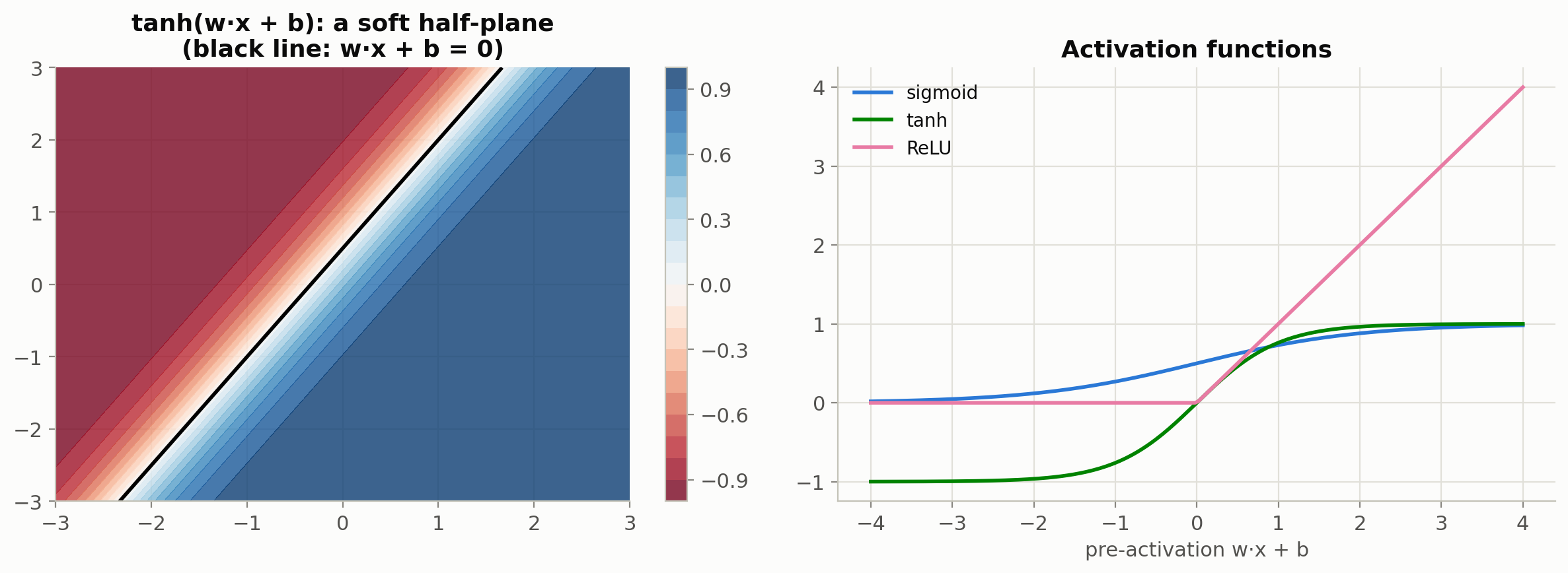
A neuron computes w · x + b — a weighted vote over its inputs plus an offset — and passes the result through a nonlinearity. That’s it. With 2 inputs, w · x + b = 0 is a line; the neuron’s output says how far on which side a point falls.
Code
w = np.array([1.5, -1.0]) # weights: one per inputb =0.5# bias: shifts the line off the origindef neuron(x, activation=np.tanh):return activation(x @ w + b)x = np.array([1.0, 2.0])print(f'pre-activation w·x + b = {x @ w + b:+.2f}')print(f'after tanh = {neuron(x):+.2f}')
pre-activation  w·x + b = +0.00
after tanh              = +0.00
Plot: the neuron’s half-plane, and three activations
One neuron = one line. Every decision it can express is “which side of my line are you on, and by how much”. To draw anything curvier, we need to combine neurons — and for that, the nonlinearity is load-bearing.
2. Why the nonlinearity is not optional
Stack two linear layers (no activation) and you get… one linear layer. The composition of matrix multiplies is a matrix multiply: (x @ W1) @ W2 = x @ (W1 @ W2). Depth without nonlinearity buys exactly nothing:
Code
W1 = rng.normal(size=(2, 8))W2 = rng.normal(size=(8, 1))x_batch = rng.normal(size=(5, 2))two_layers = (x_batch @ W1) @ W2 # "deep" linear networkone_layer = x_batch @ (W1 @ W2) # single equivalent matrixprint('max |two_layers - one_layer| =', np.abs(two_layers - one_layer).max())print('The 2-8-1 linear net IS the 2-1 matrix W1 @ W2 — still a single line.')
max |two_layers - one_layer| = 8.881784197001252e-16
The 2-8-1 linear net IS the 2-1 matrix W1 @ W2 — still a single line.
3. XOR: the smallest problem one neuron cannot solve
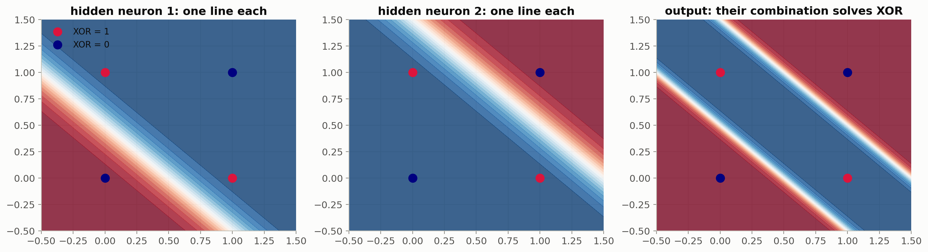
XOR’s positive examples sit on opposite corners — no single line separates them (Minsky & Papert’s 1969 objection to the perceptron). Two tanh neurons plus a combiner do it: one neuron draws each line, the combiner ANDs the two half-planes. Weights below are set by hand — learning them is the next two chapters.
Code
# Hidden neuron 1: fires above the line x1 + x2 = 0.5 ("at least one input on")# Hidden neuron 2: fires below the line x1 + x2 = 1.5 ("not both inputs on")Wh = np.array([[ 4.0, 4.0], [-4.0, -4.0]]).T # (2 inputs, 2 hidden)bh = np.array([-2.0, 6.0])wo = np.array([3.0, 3.0]) # AND the two half-planesbo =-3.0def xor_mlp(x): h = np.tanh(x @ Wh + bh) # (n, 2) hidden activationsreturn np.tanh(h @ wo + bo) # (n,) outputX_xor = np.array([[0., 0.], [0., 1.], [1., 0.], [1., 1.]])for xi, target inzip(X_xor, [0, 1, 1, 0]):print(f' x = {xi} → {xor_mlp(xi[None])[0]:+.2f} (XOR: {target})')
  x = [0. 0.]  →  -0.99   (XOR: 0)
  x = [0. 1.]  →  +0.99   (XOR: 1)
  x = [1. 0.]  →  +0.99   (XOR: 1)
  x = [1. 1.]  →  -0.99   (XOR: 0)
Plot: the two hidden half-planes and their combination
Running each neuron separately is a loop over dot products. Stacking every neuron’s w as a column of a matrix turns the whole layer — over a whole batch — into one matrix multiplication. This notation carries the entire book: attention, FFNs, the output head are all x @ W at heart (see it in 3D in the Transformer Overview):
Code
batch = rng.normal(size=(32, 2)) # (batch, n_in) 32 points, 2 featuresW = rng.normal(size=(2, 8)) / np.sqrt(2) # (n_in, n_out) 8 neurons' weights, as columnsb_vec = np.zeros(8) # (n_out,) one bias per neuronhidden = np.tanh(batch @ W + b_vec) # (32, 2) @ (2, 8) -> (32, 8)print(f'input {batch.shape} @ W {W.shape} -> hidden {hidden.shape}')print('One matmul = every neuron applied to every example at once.')print('This is why GPUs (matmul machines) and neural nets get along so well.')
input   (32, 2)   @   W (2, 8)   ->   hidden (32, 8)
One matmul = every neuron applied to every example at once.
This is why GPUs (matmul machines) and neural nets get along so well.
5. Depth and width: what random networks already do
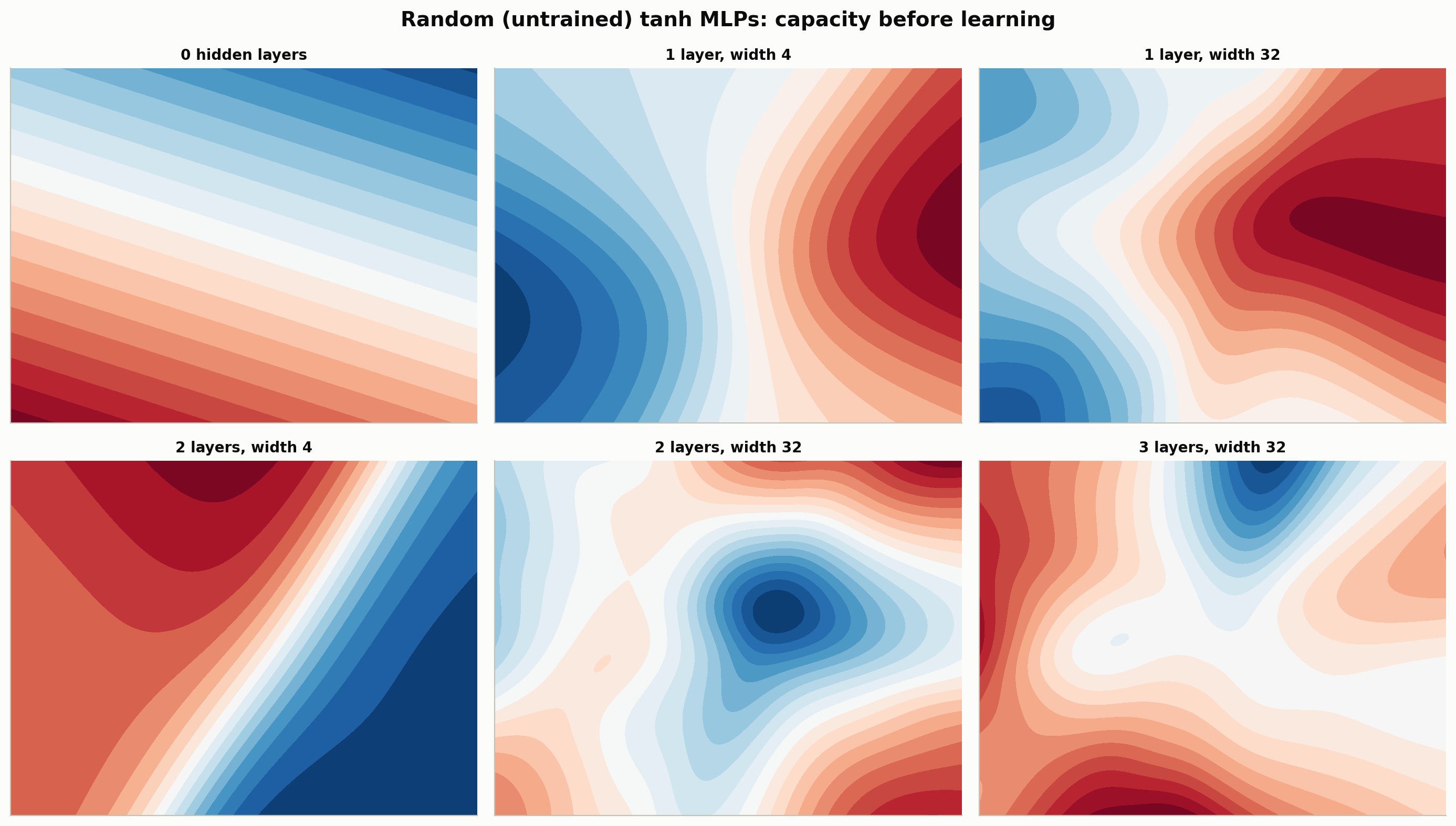
An MLP with enough hidden units can approximate any continuous function (Cybenko, 1989) — width buys expressiveness, depth buys it cheaply (features composed of features). You can see the raw material even with random, untrained weights: deeper/wider nets carve wigglier regions out of the plane.
Plot: random-weight MLPs of increasing depth and width
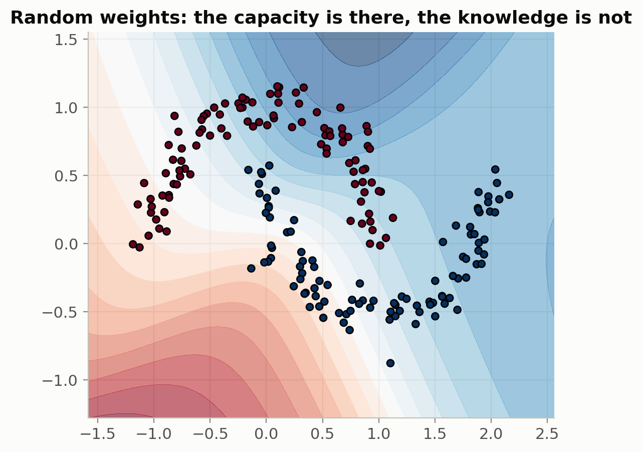
ai_playground.fundamentals.datasets.make_moons gives two interleaved arcs: not linearly separable, easily solved by a small MLP — if the weights are right. With random weights, the boundary is confidently, uselessly wrong:
Code
from ai_playground.fundamentals import make_moons, plot_decision_boundaryX, y = make_moons(n=200, noise=0.1, seed=0)f = random_mlp_fn([2, 8, 1], seed=3)ax = plot_decision_boundary(f, X, y)ax.set_title('Random weights: the capacity is there, the knowledge is not')plt.show()
Key Takeaways
A neuron is w·x + b through a squash — one line’s worth of opinion about the plane.
Nonlinearity is load-bearing: stacked linear layers collapse to a single matrix ((x@W1)@W2 = x@(W1@W2)); the activation between them is what makes depth real.
A layer is a matmul — (batch, n_in) @ (n_in, n_out). All of ai_playground.models is this pattern at scale.
Capacity ≠ knowledge: random deep nets carve rich regions (Cybenko, 1989 says rich enough), but the moons boundary is garbage until the weights are learned.
Learning the weights means computing how the loss changes with each weight — the gradient. Building the machine that computes it is the next chapter: Backprop from Scratch.