Softmax, Cross-Entropy, and Your First Classifier (M0)
The refresher’s finale connects the loop to the loss every LLM trains with. An LLM is a classifier over its vocabulary — at each position it scores 32K–128K candidate tokens, and those scores are trained with exactly what this chapter builds:
Softmax — scores to probabilities, with temperature and a stability trick
Cross-entropy — the “surprise” loss, and why MSE is the wrong tool
The p − y gradient — derived by the chapter-01 engine, verified against PyTorch
Milestone M0 — train an MLP classifier from scratch on the 3-class spiral
Concepts covered
#
Concept
What to watch for
1
Softmax
exp-and-normalize; temperature reshapes, subtract-max stabilizes
2
Cross-entropy
−log p(correct): cheap when right, catastrophic when confidently wrong
3
CE vs MSE
MSE’s gradient vanishes exactly where learning is most needed
4
p − y
The gradient at the logits is just probabilities minus targets
5
Logits → loss
The same pipeline as the LLM output head, at vocab_size = 3
Your capstone LLM’s output head is this chapter with more columns: hidden states meet a (dim, vocab_size) matrix, softmax turns the scores into a next-token distribution, and cross-entropy on the correct token is the entire training signal (the loss deep-dive traces the tensor shapes). Even generation is here: generate_tiny in the Transformer Overview is softmax + temperature + sampling, verbatim.
This chapter closes the refresher by doing the whole pipeline at vocab_size = 3 — small enough to check every number by hand, identical in shape to the real thing.
🏗️ Chapter milestone: M0 — train an MLP classifier from scratch (end of this chapter): your engine’s gradients matched against PyTorch to 1e-6, and a spiral classifier at ≥95% accuracy.
Tip⏱️ Sessions S0.4–S0.5
Two sessions: S0.4 reads the chapter; S0.5 is 🏗️ milestone M0 — the classifier trained with your own engine. Cards, prerequisites, and done-when tests: the Session Guide.
Setup
# Setup — works from a repo checkout (via ../src) or standalone on Colabimport syssys.path.insert(0, '../src')try:import ai_playground # noqa: F401exceptImportError:%pip install -q git+https://github.com/ggreg/ai_playground.git%config InlineBackend.figure_format ='retina'from ai_playground.plotting import apply_plot_styleapply_plot_style()
Code
import matplotlib.pyplot as pltimport numpy as npimport torchimport torch.nn.functional as Ffrom ai_playground.fundamentals import Value, make_spiral
1. Softmax: scores to probabilities
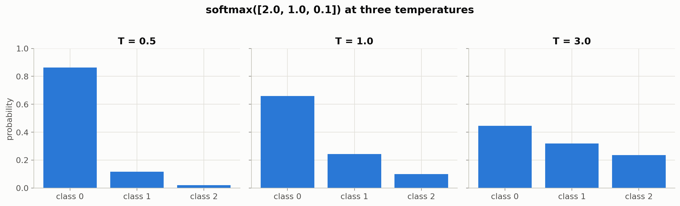
A model’s raw outputs (logits) are unbounded scores. Softmax — exp each score, divide by the sum — turns them into a probability distribution that keeps the ranking while making the confidence explicit. Temperature divides the logits first: T < 1 sharpens toward argmax, T > 1 flattens toward uniform. This is the same T you set when sampling from an LLM.
Code
def softmax(z, temperature=1.0): z = np.asarray(z, dtype=np.float64) / temperature e = np.exp(z - z.max()) # subtract-max: see belowreturn e / e.sum()logits = np.array([2.0, 1.0, 0.1])fig, axes = plt.subplots(1, 3, figsize=(13, 3.8), sharey=True)for ax, T inzip(axes, [0.5, 1.0, 3.0]): ax.bar(['class 0', 'class 1', 'class 2'], softmax(logits, T)) ax.set_title(f'T = {T}') ax.set_ylim(0, 1)axes[0].set_ylabel('probability')fig.suptitle('softmax([2.0, 1.0, 0.1]) at three temperatures', y=1.02)plt.tight_layout()plt.show()
Code
# Why subtract the max: exp overflows float64 near z = 710, and LLM logits can spike.z = np.array([1000.0, 999.0, 0.0])with np.errstate(over='ignore', invalid='ignore'): naive = np.exp(z) / np.exp(z).sum()print('naive softmax([1000, 999, 0]) =', naive) # nan — exp(1000) = infprint('stable (subtract max) version =', softmax(z))# Softmax is shift-invariant — softmax(z) == softmax(z - c) — so subtracting max(z)# changes nothing mathematically and everything numerically.
naive softmax([1000, 999, 0])  = [nan nan  0.]
stable (subtract max) version = [0.73105858 0.26894142 0.        ]
2. Cross-entropy: the surprise loss
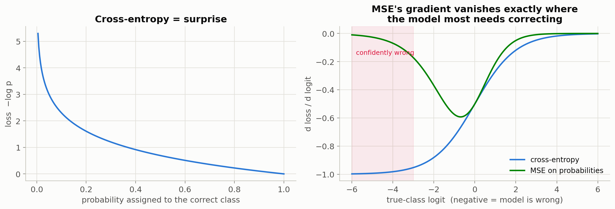
Cross-entropy scores a prediction by the log of the probability it assigned to the truth: L = −log p(correct). Read it as surprise: p = 0.99 costs 0.01 nats, p = 0.01 costs 4.6. And its gradient is exactly what a learning signal should be — compare what happens to MSE-on-probabilities when the model is confidently wrong:
Plot: −log p, and CE vs MSE gradients when the model is wrong
fig, axes = plt.subplots(1, 2, figsize=(12, 4.2))p = np.linspace(0.005, 1.0, 300)axes[0].plot(p, -np.log(p))axes[0].set_xlabel('probability assigned to the correct class')axes[0].set_ylabel('loss −log p')axes[0].set_title('Cross-entropy = surprise')# Two classes, true class 0: sweep the true-class logit z (other fixed at 0)# and plot dL/dz for CE vs MSE-on-softmax, computed by torch autograd.zs = np.linspace(-6, 6, 200)grads = {'cross-entropy': [], 'MSE on probabilities': []}for z0 in zs:for name in grads: zt = torch.tensor([z0, 0.0], requires_grad=True) probs = torch.softmax(zt, dim=0) loss = (-torch.log(probs[0]) if name =='cross-entropy'else ((probs - torch.tensor([1.0, 0.0])) **2).sum()) loss.backward() grads[name].append(zt.grad[0].item())for name, g in grads.items(): axes[1].plot(zs, g, label=name)axes[1].axvspan(-6, -3, color='crimson', alpha=0.08)axes[1].text(-5.8, -0.15, 'confidently wrong', fontsize=9, color='crimson')axes[1].set_xlabel('true-class logit (negative = model is wrong)')axes[1].set_ylabel('d loss / d logit')axes[1].legend()axes[1].set_title("MSE's gradient vanishes exactly where\nthe model most needs correcting")plt.tight_layout()plt.show()
That red zone is the argument: with MSE on probabilities, a very wrong model gets a near-zero gradient (the softmax has saturated) and learns nothing. Cross-entropy’s gradient stays large until the model is actually right. The deeper reason it’s the LLM loss — maximum likelihood over the vocabulary — is in docs/CONCEPTS.md.
3. The famous gradient: p − y
Push one sample through softmax + cross-entropy with the chapter-01 engine — its exp and log are all we need — and read the logit gradients off the graph. The claimed closed form: probabilities minus one-hot target.
Code
logits = [Value(2.0), Value(1.0), Value(0.1)]target =0# true classexps = [z.exp() for z in logits]total = exps[0] + exps[1] + exps[2]probs = [e / total for e in exps]loss =-(probs[target].log()) # cross-entropy, built from scratchloss.backward()p_np = softmax([2.0, 1.0, 0.1])y_onehot = np.eye(3)[target]print(f'{"class":>5}{"engine dL/dz":>13}{"p − y":>13}')for k inrange(3):print(f'{k:>5}{logits[k].grad:>13.8f}{p_np[k] - y_onehot[k]:>13.8f}')# And against torch.nn.functional.cross_entropy (which fuses all of the above):zt = torch.tensor([[2.0, 1.0, 0.1]], requires_grad=True)F.cross_entropy(zt, torch.tensor([target])).backward()assert np.allclose([z.grad for z in logits], zt.grad[0].numpy(), atol=1e-6)print('\nmatches F.cross_entropy grads to 1e-6 ✓')
class   engine dL/dz          p − y
    0    -0.34099886    -0.34099886
    1     0.24243297     0.24243297
    2     0.09856589     0.09856589

matches F.cross_entropy grads to 1e-6 ✓
p − y is worth memorizing: the entire softmax + log + normalize pipeline collapses to “how much probability did you put where it didn’t belong”. It’s also why frameworks fuse softmax into the loss (F.cross_entropy takes logits) — the fused backward is this one subtraction, with none of the intermediate graph.
4. M0’s task: the 3-class spiral
make_spiral interleaves three arms — the CS231n classic. First, proof that our engine can learn it (briefly, on a subset — scalar autograd pays per node), then the full run in PyTorch:
Code
from ai_playground.fundamentals import MLP, plot_decision_boundaryX, y = make_spiral(n_per_class=100, n_classes=3, noise=0.2, seed=0)# --- scalar engine, small slice: prove the machinery learns ---idx = np.random.default_rng(0).permutation(len(X))[:60]Xs, ys = X[idx], y[idx]m = MLP(2, [8, 3], seed=2)def ce_loss(model, Xb, yb): total =Nonefor xi, yi inzip(Xb, yb): zs = model([*xi]) exps = [z.exp() for z in zs] denom = exps[0] + exps[1] + exps[2] nll =-((exps[int(yi)] / denom).log()) total = nll if total isNoneelse total + nllreturn total /len(Xb)start = ce_loss(m, Xs, ys).datafor step inrange(150): loss = ce_loss(m, Xs, ys) m.zero_grad(); loss.backward()for p in m.parameters(): p.data -=2.0* p.gradacc = np.mean([int(np.argmax([z.data for z in m([*xi])])) == yi for xi, yi inzip(Xs, ys)])print(f'scalar engine on 60 points: CE {start:.3f} -> {ce_loss(m, Xs, ys).data:.3f}, 'f'accuracy {acc:.0%} (chance: 33%)')print('The engine learns — now let torch handle the full 300 points at speed.')
scalar engine on 60 points: CE 1.098 -> 0.449, accuracy 77% (chance: 33%)
The engine learns — now let torch handle the full 300 points at speed.
Code
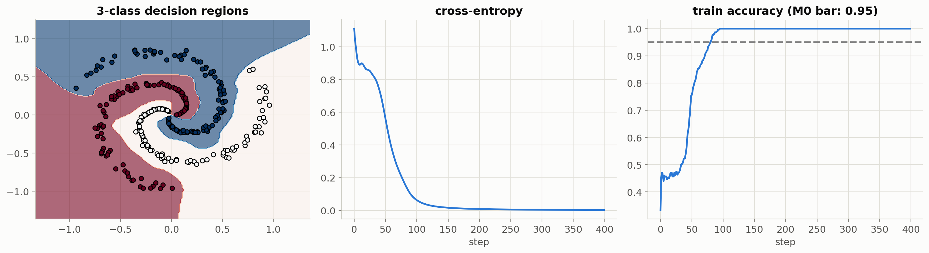
# --- PyTorch, full 300 points ---tmodel = torch.nn.Sequential(torch.nn.Linear(2, 32), torch.nn.Tanh(), torch.nn.Linear(32, 32), torch.nn.Tanh(), torch.nn.Linear(32, 3))opt = torch.optim.Adam(tmodel.parameters(), lr=0.01)tX, ty = torch.tensor(X, dtype=torch.float32), torch.tensor(y)curve, acc_curve = [], []for step inrange(400): logits_t = tmodel(tX) loss = F.cross_entropy(logits_t, ty) # fused softmax + CE, gradient p − y curve.append(loss.item()) acc_curve.append((logits_t.argmax(1) == ty).float().mean().item()) opt.zero_grad(); loss.backward(); opt.step()train_acc = acc_curve[-1]print(f'final CE {curve[-1]:.4f}, train accuracy {train_acc:.1%} on 300 points')
final CE 0.0022, train accuracy 100.0% on 300 points
Swap the spiral’s 2 features for dim-dimensional hidden states and its 3 classes for a vocabulary, and nothing else changes: the LLM output head is h @ W_out into F.cross_entropy, gradient p − y over vocab_size entries per position. That single matmul is visualized in 3D in the Transformer Overview (§4b), and the full tensor-shape walk lives in docs/CONCEPTS.md § loss function. What changes at scale is only engineering: at vocab 128K the logits row is the biggest tensor in the step, which is why fused softmax-CE kernels exist.
🏗️ Project milestone M0 — train an MLP classifier from scratch
Close the refresher by proving both halves of it on your own machine: your engine’s gradients are correct, and the loop they power actually learns.
from pathlib import PathWS = Path('../../checkpoints/myllm')WS.mkdir(parents=True, exist_ok=True)
Gradient parity — build one spiral batch (16 points), compute softmax + CE with ai_playground.fundamentals (Value, MLP(2, [8, 3])) and with an identical-weight torch model (the weight-copy recipe is in tests/test_fundamentals.py::TestMLP::test_grad_parity_with_torch). Record the max absolute gradient difference.
Spiral accuracy — train any MLP you like (torch allowed — the loop is chapter 02’s) on the full 300-point spiral; record final train accuracy.
Accept when: m0_grad_max_abs_diff < 1e-6, m0_spiral_train_acc >= 0.95, and both keys are in metrics.json. Part of The Project: Serve Your Own LLM.
Session S0.5 — verify: uv run pytest tests/milestones/test_m00_classifier.py.
Key Takeaways
Softmax = exp-and-normalize, temperature reshapes confidence, and subtract-max costs nothing (shift invariance) while preventing overflow — the reason every real implementation does it.
Cross-entropy is surprise, and its gradient survives where MSE’s dies: a confidently-wrong model gets a full-strength correction instead of a saturated zero.
p − y — the whole softmax+CE backward collapses to probabilities minus targets, derived here by the scalar engine and matched to F.cross_entropy at 1e-6.
An LLM is this classifier with a huge class count: same head, same loss, same gradient, per token position.
M0 done means the refresher’s promise is kept: an engine you built, verified against PyTorch, driving a loop you understand, hitting ≥95% on a task a linear model cannot touch. The main path resumes at the Transformer Overview — where milestone M1 designs the model this classifier grows into.
🔨 From-scratch project: p0 — Autograd from a blank file
You’ve now run every piece of the refresher — and the M0 milestone had you re-apply the repo’s engine. The phase’s from-scratch project asks for more: rebuild the whole stack (scalar autograd, an MLP, a training loop that separates the moons) with nothing open but a blank file. Scaffolding covers the boilerplate; the acceptance tests check your gradients against central finite differences, not against any library.