CUDA Basics: GPU Memory Hierarchy, Warps, and Occupancy
This notebook builds the mental model you need before reading kernel code (Triton, FlashAttention, custom CUDA) or interpreting profiler output. We’ll cover what a GPU actually is, why memory hierarchy dominates LLM performance, and how the execution model (threads → warps → blocks → grid) maps to the hardware.
By the end, you should be able to answer:
Why is FlashAttention faster than vanilla attention if it does more FLOPs? (Dao et al., 2022)
Why does a 7B-param LLM at long context become memory-bandwidth-bound, not compute-bound, during decode?
What does “MFU = 45%” actually measure, and why is 100% impossible? (See src/ai_playground/profiling/flops.py.)
Concepts covered
#
Concept
Section
1
GPU vs CPU: throughput vs latency hardware
§1
2
Memory hierarchy (registers → SRAM → L2 → HBM)
§2
3
Bandwidth wall and the roofline model
§3
4
SIMT execution: threads, warps, blocks, grids
§4
5
Occupancy and latency hiding
§5
6
Writing a first CUDA kernel (Numba)
§6
7
Coalesced memory access
§7
8
Why this matters for LLMs (FlashAttention, GEMM, MFU)
Build the GPU mental model: memory hierarchy, warps, occupancy, coalescing — and why LLM decode is bandwidth-bound.
🏗️ Chapter milestone: M9 — place your model’s decode on the T4 roofline — the exercise at the end of this chapter; see The Project.
Tip⏱️ Sessions S5.1–S5.2
Two sessions: S5.1 builds the GPU mental model; S5.2 is 🏗️ M9 — your model’s decode roofline. Cards, prerequisites, and done-when tests: the Session Guide.
The kernel cells need an NVIDIA GPU: on Colab pick Runtime → Change runtime type → T4 GPU. Without one, the notebook still runs — kernel cells fall back to illustrations.
Setup
# Setup — works from a repo checkout (via ../src) or standalone on Colabimport syssys.path.insert(0, '../src')try:import ai_playground # noqa: F401exceptImportError:%pip install -q git+https://github.com/ggreg/ai_playground.git%config InlineBackend.figure_format ='retina'from ai_playground.plotting import apply_plot_styleapply_plot_style()
Code
import syssys.path.insert(0, '../src')import torchimport numpy as npimport matplotlib.pyplot as plttorch.manual_seed(42)device ='cuda'if torch.cuda.is_available() else'mps'if torch.backends.mps.is_available() else'cpu'HAS_CUDA = torch.cuda.is_available()print(f'Device: {device}')if HAS_CUDA:print(f'GPU: {torch.cuda.get_device_name(0)}')print(f'Compute capability: {torch.cuda.get_device_capability(0)}')else:print('No CUDA GPU — kernel cells will be illustrative.')print('To run for real: see docs/CLOUD_SETUP.md.')
Device: mps
No CUDA GPU — kernel cells will be illustrative.
To run for real: see docs/CLOUD_SETUP.md.
1. GPU vs CPU: throughput vs latency hardware
A modern CPU core is optimized to finish one sequential thread fast: deep pipelines, branch prediction, large per-core caches, out-of-order execution. A GPU SM (Streaming Multiprocessor) is the opposite — it’s optimized to keep thousands of threads in flight so it can hide memory latency by always having other work to do.
Concrete numbers (H100 SXM vs a high-end CPU):
CPU (e.g. EPYC 9654)
H100 SXM
Cores / SMs
96 cores
132 SMs
Threads in flight
~192 (2 per core)
~270,000 (2,048 per SM)
Peak FP32 throughput
~5 TFLOPS
67 TFLOPS
Peak BF16 tensor cores
—
989 TFLOPS
Memory bandwidth
~460 GB/s (DDR5)
3,350 GB/s (HBM3)
The GPU has ~7x the bandwidth and ~200x the BF16 throughput, but each individual thread is slower than a CPU thread. GPUs win by parallelism, not single-thread speed.
This shapes everything that follows. If you can’t expose enough parallel work, or if your work pattern fights the memory system, you’ll get a fraction of peak.
2. Memory hierarchy
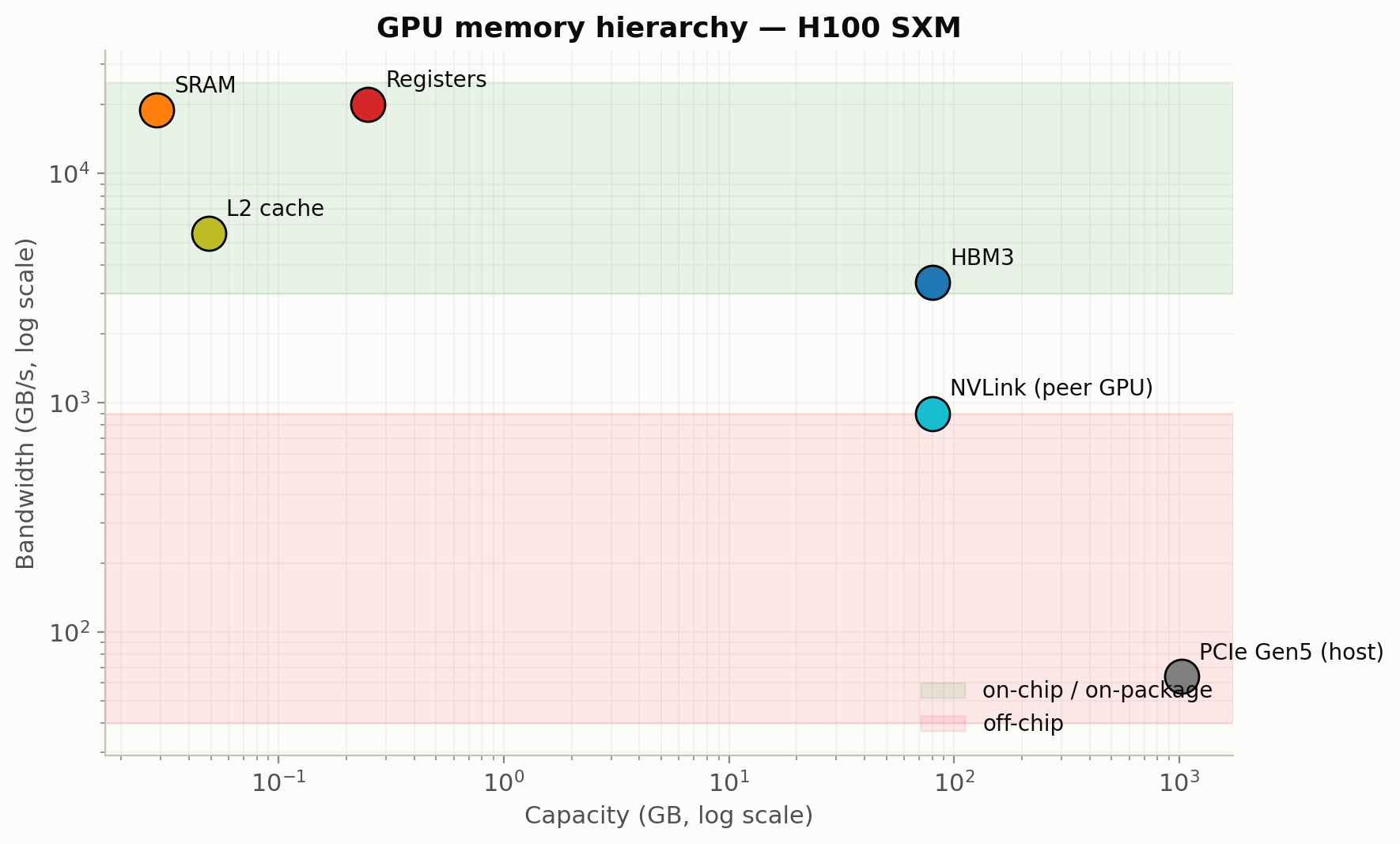
The most important fact about a GPU isn’t its FLOPS — it’s that memory is structured as a hierarchy with orders-of-magnitude bandwidth differences between levels. Understanding this is the difference between “my kernel is slow and I don’t know why” and “I can read FlashAttention and explain every choice.”
For an H100:
Level
Size
Bandwidth
Latency
Scope
Registers
256 KB / SM
~20 TB/s effectively
~1 cycle
per-thread
Shared memory (SRAM)
228 KB / SM
~19 TB/s
~30 cycles
per-block
L2 cache
50 MB
~5.5 TB/s
~200 cycles
device-wide
HBM (global memory)
80 GB
3.35 TB/s
~500 cycles
device-wide
A few takeaways:
SRAM is ~6x faster than HBM. This is the single number behind FlashAttention’s ~2-4x speedup: it tiles attention so Q, K, V tiles live in SRAM during the softmax+matmul, instead of the whole n × n score matrix being written to HBM.
Registers are private to a thread. They hold the values you’re actively computing on.
Shared memory is per-block, programmer-managed. Unlike CPU cache, you decide what goes there. This is the main lever for kernel optimization.
HBM is huge but slow. Every load from global memory is ~500 cycles of latency. Hiding this latency requires having lots of other warps ready to run (§5).
Code
# Visualize the memory hierarchy: capacity (log) vs bandwidth (log).levels = [ ('Registers', 256/1024, 20_000, 'tab:red'), # GB, GB/s ('SRAM', 228/1024/1024*132, 19_000, 'tab:orange'), ('L2 cache', 50/1024, 5_500, 'tab:olive'), ('HBM3', 80, 3_350, 'tab:blue'), ('NVLink (peer GPU)', 80, 900, 'tab:cyan'), ('PCIe Gen5 (host)', 1024, 64, 'tab:gray'),]fig, ax = plt.subplots(figsize=(9, 5.5))for name, cap_gb, bw_gbs, color in levels: ax.scatter(cap_gb, bw_gbs, s=240, color=color, edgecolor='black', zorder=3) ax.annotate(name, (cap_gb, bw_gbs), xytext=(8, 8), textcoords='offset points', fontsize=10)ax.set_xscale('log'); ax.set_yscale('log')ax.set_xlabel('Capacity (GB, log scale)')ax.set_ylabel('Bandwidth (GB/s, log scale)')ax.set_title('GPU memory hierarchy — H100 SXM')ax.grid(True, which='both', alpha=0.3)ax.axhspan(3000, 25000, alpha=0.08, color='green', label='on-chip / on-package')ax.axhspan(40, 900, alpha=0.08, color='red', label='off-chip')ax.legend(loc='lower right')plt.tight_layout()plt.show()print('Rule of thumb: every step DOWN the hierarchy is ~5-10x slower bandwidth.')print('A kernel that touches HBM 10x more than necessary will be ~10x slower than it should be.')
Rule of thumb: every step DOWN the hierarchy is ~5-10x slower bandwidth.
A kernel that touches HBM 10x more than necessary will be ~10x slower than it should be.
3. The bandwidth wall and the roofline model
Whether a kernel is compute-bound or memory-bound depends on its arithmetic intensity:
\[\text{AI} = \frac{\text{FLOPs performed}}{\text{bytes moved from HBM}}\]
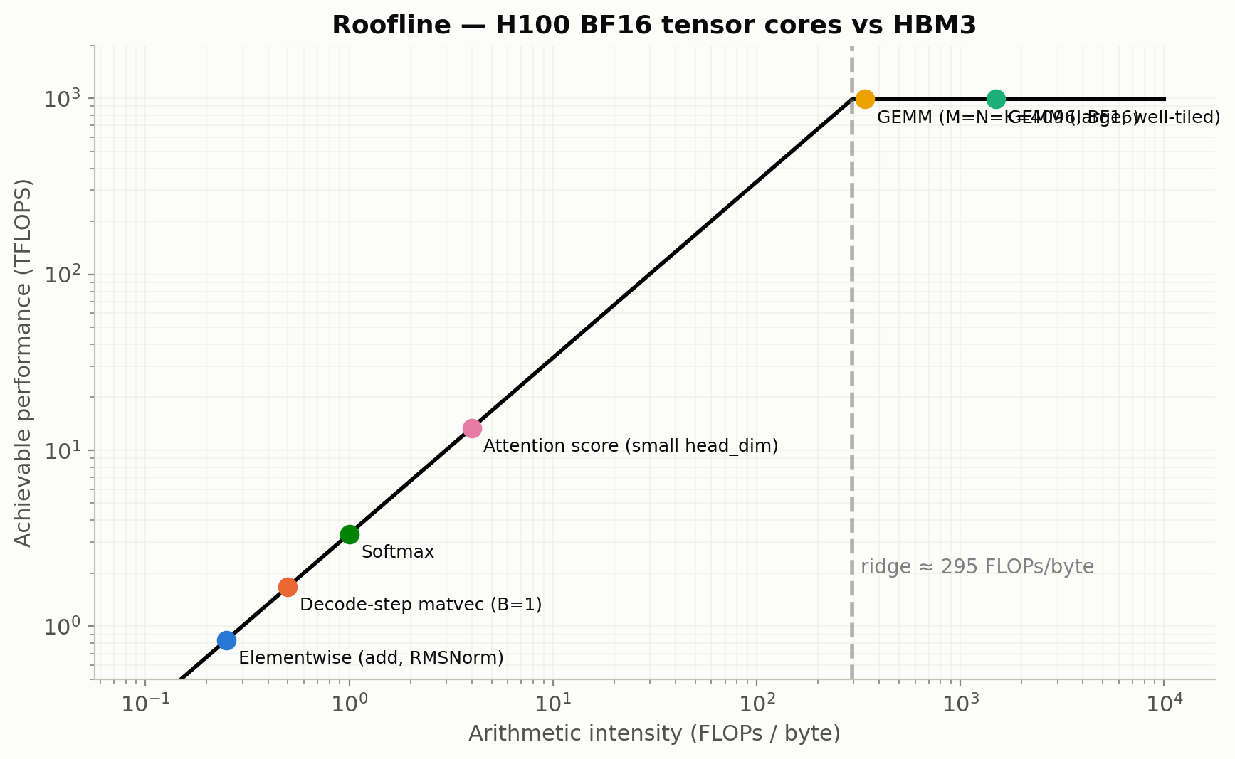
The roofline model (Williams et al., 2009) plots achievable performance vs arithmetic intensity. Below the “ridge point”, you’re limited by bandwidth (AI × peak_BW); above it, by peak FLOPS.
For an H100 (BF16 tensor cores, 989 TFLOPS peak, 3,350 GB/s HBM):
So you need ~295 FLOPs per byte read from HBM just to not be bandwidth-bound. That’s a high bar.
Code
# Roofline plot for H100 BF16, with common LLM ops marked.peak_tflops =989# BF16 tensor corespeak_bw_tbs =3.35# HBM3ridge = peak_tflops / peak_bw_tbsai = np.logspace(-1, 4, 500)perf = np.minimum(ai * peak_bw_tbs, peak_tflops)ops = [# (label, arithmetic intensity FLOPs/byte, achieved-ish TFLOPS) ('Elementwise (add, RMSNorm)', 0.25, None), ('Softmax', 1.0, None), ('Attention score (small head_dim)', 4.0, None), ('GEMM (M=N=K=4096, BF16)', 340, None), ('GEMM (large, well-tiled)', 1500, None), ('Decode-step matvec (B=1)', 0.5, None), # purely memory bound]fig, ax = plt.subplots(figsize=(9, 5.5))ax.loglog(ai, perf, 'k-', linewidth=2)ax.axvline(ridge, color='gray', linestyle='--', alpha=0.6)ax.text(ridge *1.1, 2, f'ridge ≈ {ridge:.0f} FLOPs/byte', fontsize=10, color='gray')for label, x, _ in ops: y =min(x * peak_bw_tbs, peak_tflops) ax.scatter(x, y, s=80, zorder=3) ax.annotate(label, (x, y), xytext=(6, -12), textcoords='offset points', fontsize=9)ax.set_xlabel('Arithmetic intensity (FLOPs / byte)')ax.set_ylabel('Achievable performance (TFLOPS)')ax.set_title('Roofline — H100 BF16 tensor cores vs HBM3')ax.grid(True, which='both', alpha=0.3)ax.set_ylim(0.5, 2000)plt.tight_layout()plt.show()print('Notice: most LLM ops EXCEPT large GEMMs are bandwidth-bound on modern GPUs.')print('This is why fusing elementwise ops (RMSNorm + residual + ...) matters so much.')print('It is also why decode (B=1) tops out at ~5-10% MFU even for perfect kernels.')
Notice: most LLM ops EXCEPT large GEMMs are bandwidth-bound on modern GPUs.
This is why fusing elementwise ops (RMSNorm + residual + ...) matters so much.
It is also why decode (B=1) tops out at ~5-10% MFU even for perfect kernels.
CUDA’s programming model is SIMT (Single Instruction, Multiple Threads). You write code from the perspective of one thread, but the hardware runs them in lockstep groups.
grid          = many blocks (your problem, e.g. 1M elements)
  └── block   = group of threads scheduled together on one SM (e.g. 256 threads)
        └── warp = 32 threads executing the same instruction in lockstep
              └── thread = one execution lane, with its own registers
Key facts:
A warp is always 32 threads on NVIDIA hardware. This is a hardware constant, not a tuning knob.
All 32 threads in a warp execute the same instruction every cycle. If they branch differently (if/else), the GPU executes both paths serially with the inactive lanes masked out — this is “warp divergence” and it costs performance.
Blocks are scheduled to one SM and can use shared memory to cooperate. Threads in different blocks can’t share fast memory — only HBM or atomics.
Block size should be a multiple of 32. Common choices: 128, 256, 512. Below 32 wastes lanes; above 1024 isn’t allowed.
When you write kernel<<<grid_dim, block_dim>>>(...) you’re saying: launch grid_dim × block_dim total threads, organized as grid_dim blocks of block_dim threads each.
5. Occupancy and latency hiding
Recall HBM latency is ~500 cycles. If a warp issues a load, what does the SM do for the next 500 cycles? It runs other warps. That’s the entire trick.
Occupancy = (active warps per SM) / (max warps per SM). On an H100, max is 64 warps/SM = 2,048 threads/SM. Higher occupancy generally hides memory latency better — but there are tradeoffs:
Registers per thread is finite (255 max, ~64K total per SM). More registers per thread → fewer threads can fit → lower occupancy.
Shared memory per block is finite (228 KB on H100). Bigger tiles → fewer blocks per SM → lower occupancy.
Higher occupancy isn’t always better. Volkov’s classic talk “Better Performance at Lower Occupancy” shows that for arithmetic-heavy kernels, putting more work per thread (using more registers) can beat raw occupancy.
For LLMs, the practical heuristics:
Aim for ≥50% occupancy as a starting point.
If you’re memory-bound (most of attention, RMSNorm, etc.), occupancy matters a lot.
The CUDA Occupancy Calculator and nsys/ncu (covered in 03_nsight_profiling.ipynb) will tell you what’s actually limiting you.
6. A first CUDA kernel: vector add
Let’s actually write one. Vector add is the “hello world” of GPU programming — every thread reads one element of a and b, writes one element of c. Embarrassingly parallel, ~zero arithmetic intensity, purely memory-bound.
We’ll use Numba’s @cuda.jit because it lets us stay in Python. (Triton — covered in 02_triton_kernels.ipynb — is the modern choice for production kernels, but Numba is the gentlest first step.)
The kernel runs only if you have CUDA; otherwise we describe what it would do.
Code
# Numba CUDA vector-add kernel. Falls back to a description if no CUDA.KERNEL_SRC ='''@cuda.jitdef vector_add(a, b, c): # Each thread computes one output element. # `cuda.grid(1)` returns this thread's global 1D index. i = cuda.grid(1) if i < a.size: c[i] = a[i] + b[i]'''print('Kernel source:')print(KERNEL_SRC)if HAS_CUDA:try:from numba import cudaimport numbaimport math@cuda.jitdef vector_add(a, b, c): i = cuda.grid(1)if i < a.size: c[i] = a[i] + b[i] N =1<<24# 16M elements a = np.random.randn(N).astype(np.float32) b = np.random.randn(N).astype(np.float32) c = np.zeros_like(a) d_a = cuda.to_device(a) d_b = cuda.to_device(b) d_c = cuda.to_device(c) threads_per_block =256 blocks_per_grid = math.ceil(N / threads_per_block)print(f'Launching {blocks_per_grid} blocks x {threads_per_block} threads = {blocks_per_grid * threads_per_block:,} threads')print(f' Total warps: {blocks_per_grid * threads_per_block //32:,}')# Warmup + time vector_add[blocks_per_grid, threads_per_block](d_a, d_b, d_c) cuda.synchronize() start = cuda.event(); end = cuda.event() start.record()for _ inrange(50): vector_add[blocks_per_grid, threads_per_block](d_a, d_b, d_c) end.record(); end.synchronize() ms = cuda.event_elapsed_time(start, end) /50 bytes_moved =3* N *4# read a, read b, write c — fp32 bw = bytes_moved / (ms *1e-3) /1e9print(f'\nKernel time: {ms:.3f} ms')print(f'Effective bandwidth: {bw:.1f} GB/s')print('(Compare to your GPU peak — vector add should hit 70-90% of peak HBM bandwidth.)')exceptImportError:print('Numba not installed. `uv pip install numba` to run for real.')else:print('No CUDA — but here is what would happen:')print(' - 16M elements, 256 threads/block → 65,536 blocks')print(' - Each thread reads 8 bytes (a[i] + b[i]), writes 4 bytes')print(' - Total: 12 bytes per element x 16M = 192 MB of HBM traffic')print(' - On H100 (3.35 TB/s): theoretical minimum ~57 microseconds')print(' - Real kernels typically achieve 70-90% of peak bandwidth.')
Kernel source:

@cuda.jit
def vector_add(a, b, c):
    # Each thread computes one output element.
    # `cuda.grid(1)` returns this thread's global 1D index.
    i = cuda.grid(1)
    if i < a.size:
        c[i] = a[i] + b[i]

No CUDA — but here is what would happen:
  - 16M elements, 256 threads/block → 65,536 blocks
  - Each thread reads 8 bytes (a[i] + b[i]), writes 4 bytes
  - Total: 12 bytes per element x 16M = 192 MB of HBM traffic
  - On H100 (3.35 TB/s): theoretical minimum ~57 microseconds
  - Real kernels typically achieve 70-90% of peak bandwidth.
7. Coalesced memory access — the single biggest performance lever
Here’s the rule that catches everyone: threads in a warp should access consecutive memory addresses.
When a warp issues a load, the memory system fetches a 128-byte cache line (or 32-byte sector). If all 32 threads request bytes within that line, the load takes one transaction — coalesced. If each thread requests a far-apart address (strided/random), it takes up to 32 transactions — 32x more bandwidth burned.
This is why layout matters as much as the algorithm. A matrix stored row-major and accessed column-by-column will be uncoalesced and ~10x slower than the row-by-row version that does the same work.
Concrete LLM example: when KV cache is laid out as (layer, batch, head, seq, dim) vs (layer, batch, seq, head, dim), the access pattern during decode determines whether reads coalesce. PagedAttention (Kwon et al., 2023) goes further and pages the cache like virtual memory, sacrificing some coalescing for much better packing — a deliberate tradeoff.
Code
# Demonstrate stride cost: copying a contiguous tensor vs. materializing# its transpose. Both move the same N*N elements; only the access pattern differs.# The transposed copy must read with stride N, which uncoalesces every warp.import timeN =8192x = torch.randn(N, N, device=device)def sync():if device =='cuda': torch.cuda.synchronize()elif device =='mps': torch.mps.synchronize()def bench(fn, runs=30, warmup=5):for _ inrange(warmup): fn() sync() t0 = time.perf_counter()for _ inrange(runs): fn() sync()return (time.perf_counter() - t0) / runs *1000# msms_contig = bench(lambda: x.clone()) # coalesced readsms_strided = bench(lambda: x.t().contiguous()) # strided reads, same byte volumebytes_moved =2* N * N *4# read + write, fp32bw_contig = bytes_moved / (ms_contig *1e-3) /1e9bw_strided = bytes_moved / (ms_strided *1e-3) /1e9print(f'clone (contiguous): {ms_contig:6.2f} ms -> {bw_contig:7.1f} GB/s effective')print(f't().contiguous (strided): {ms_strided:6.2f} ms -> {bw_strided:7.1f} GB/s effective')print(f'Slowdown: {ms_strided / ms_contig:.1f}x (same bytes moved, different access pattern)')print('\nThe strided version reads one element per cache line instead of 16 (fp32) or 32 (fp16).')print('Same lesson on CUDA: a hand-rolled transpose that does not stage through shared memory')print('to coalesce reads will hit the same cliff.')
clone (contiguous):         1.48 ms  ->    363.6 GB/s effective
t().contiguous (strided):  33.78 ms  ->     15.9 GB/s effective
Slowdown: 22.9x  (same bytes moved, different access pattern)

The strided version reads one element per cache line instead of 16 (fp32) or 32 (fp16).
Same lesson on CUDA: a hand-rolled transpose that does not stage through shared memory
to coalesce reads will hit the same cliff.
8. Why this matters for LLMs
We can now answer the questions from the intro:
Why is FlashAttention faster despite doing more FLOPs? Vanilla attention writes the n × n score matrix to HBM, runs softmax, reads it back, multiplies by V. That’s O(n²) HBM traffic. FlashAttention tiles Q, K, V so each tile fits in SRAM (§2 — ~6x faster than HBM), runs an online softmax across tiles, and never materializes the full score matrix. It does ~25% more arithmetic but cuts HBM traffic by O(n). Since attention is bandwidth-bound (§3), trading FLOPs for bandwidth wins.
Why does decode (batch=1, generating one token at a time) bottleneck on bandwidth? At batch=1, each token-generation step is a sequence of matrix–vector products, not matrix–matrix. AI ≈ 0.5 FLOPs/byte (you read all the weights for ~one FLOP per weight). Look at the roofline plot in §3: at AI=0.5, peak achievable is ~1.7 TFLOPS — barely 0.2% of an H100’s BF16 peak. You can’t fix this with a better kernel; you fix it with batching, speculative decoding, or quantization (covered in 04_inference_optimization/).
What does MFU = 45% measure? MFU = achieved FLOPs / theoretical peak FLOPS. The 55% gap comes from: bandwidth-bound ops (everything except big GEMMs), kernel launch overhead, SM occupancy below 100%, communication for distributed training, dataloader stalls, and any non-tensor-core work (FP32 reductions, softmax). State-of-the-art LLM training reaches ~40-60% — that’s the realistic ceiling, not 100%. See src/ai_playground/profiling/flops.py for the calculation.
🏗️ Project milestone M9 — your model’s decode roofline
Decode FLOPs/token ≈ 2 x num_params; decode bytes/token ≈ weight bytes + KV bytes at the current context length. Compute your model’s decode arithmetic intensity at batch 1, 8, and 32, place the three points on this chapter’s T4 roofline, and find the smallest batch where your model crosses from bandwidth-bound to compute-bound. Record the numbers in metrics.json['m9_roofline'].
Accept when: the three intensities and the crossover batch are in metrics.json, with a one-line conclusion (it should say decode at batch 1 is deeply bandwidth-bound). Part of The Project: Serve Your Own LLM.
GPUs win by parallelism, not single-thread speed. Expose enough work or you’ll get a fraction of peak.
Memory hierarchy spans ~6x bandwidth from HBM to SRAM. Most kernel optimization is “keep data in SRAM longer.” This is the FlashAttention insight (Dao et al., 2022).
Roofline tells you what to optimize. Below the ridge point, fix bandwidth. Above it, fix FLOPs. Most LLM ops outside of large GEMMs are bandwidth-bound.
Warp = 32 threads in lockstep. Block size should be a multiple of 32. Avoid divergent branches inside warps.
Latency hiding ≠ free. It needs enough warps in flight; that’s “occupancy”. 50%+ is a reasonable starting target.
Coalesce or die. Strided/random access patterns can cost 10x bandwidth. Layout choices propagate everywhere.
Decode at batch=1 is bandwidth-bound by construction — no kernel can fix it; you fix it with batching, speculation, or quantization.
MFU 40-60% is the realistic ceiling for training large models. Anything higher means you’re either lucky or measuring wrong.
What to read next
This series: 02_triton_kernels.ipynb (writing fused kernels), 03_nsight_profiling.ipynb (measuring all of the above).