Transformer Visualization: Architecture & Training from Scratch

This notebook builds a tiny transformer with a toy vocabulary of 8 words and trains it for several steps so you can watch every concept come alive:

  1. Architecture diagram β€” see how data flows through the model
  2. Single forward pass β€” trace a sentence through every layer
  3. Training loop β€” watch the loss drop and predictions improve step by step

Concepts covered

# Concept What to watch for
1 Embedding Token IDs (integers) become vectors
2 Positional encoding Same word at different positions gets different representations
8 Causal mask Each token can only see tokens before it
13 Transformer block Repeated N times β€” attention then FFN
14 Output head Vectors become next-token predictions
15 Sampling Pick the next token from the probability distribution

Reference: β€œAttention Is All You Need” Β· The Annotated Transformer Β· docs/PAPERS.md

TipπŸ“Ί Video companion

Transformers, the tech behind LLMs (3Blue1Brown) gives the visual intuition for everything built here, and Let’s build GPT (Karpathy) is the same build-it-from-scratch journey in live code β€” more in Videos.

Note🎯 Goal β€” why this chapter, for the capstone

The book’s project (The Project) ends with your own LLM served through your own inference engine. Every choice you’ll make at its first milestone β€” how wide (dim), how deep (n_layers), how many attention heads, what vocabulary β€” is a knob on the architecture this chapter takes apart.

Watching a tiny transformer assemble, train, and predict teaches what each knob does before you have to set it: the embedding table fixes the vocabulary you can serve and a big share of your parameter budget; the attention heads determine the KV cache your engine will page at the finale; the stack of blocks is the weight matrix that streams from memory on every decode step. By the end you can read the architecture diagram as a list of decisions β€”

πŸ—οΈ Chapter milestone: M1 β€” design your own model’s config under a 2M-parameter budget (the exercise at the end of this chapter). Everything later β€” training runs, roofline analysis, serving β€” builds on the config.json you write here.

Tip⏱️ Sessions S1.1–S1.2

Two sessions: S1.1 takes the model apart; S1.2 is πŸ—οΈ M1 β€” design your own config under the 2M-parameter budget. Cards, prerequisites, and done-when tests: the Session Guide.

Open in Colab

Setup
# Setup β€” works from a repo checkout (via ../src) or standalone on Colab
import sys
sys.path.insert(0, '../src')
try:
    import ai_playground  # noqa: F401
except ImportError:
    %pip install -q git+https://github.com/ggreg/ai_playground.git

%config InlineBackend.figure_format = 'retina'
from ai_playground.plotting import apply_plot_style
apply_plot_style()
Code
import sys
sys.path.insert(0, '../src')

import torch
import torch.nn as nn
import torch.nn.functional as F
import matplotlib.pyplot as plt
import matplotlib.patches as mpatches
import numpy as np
from ai_playground.models import Transformer, TransformerConfig

torch.manual_seed(42)
device = 'cpu'  # tiny model, CPU is fine

1. Our Tiny World

A vocabulary of just 8 tokens. The model’s job: learn to predict the next token.

We’ll teach it simple patterns like the cat sat on and the dog ran on.

Code
# Tiny vocabulary β€” 8 tokens total
# In real LLMs this would be 32K-128K subword tokens from BPE
# (see docs/PAPERS.md Β§ Tokenization, https://arxiv.org/abs/1508.07909)
VOCAB = ['<pad>', 'the', 'cat', 'dog', 'sat', 'ran', 'on', 'mat']
tok2id = {t: i for i, t in enumerate(VOCAB)}
id2tok = {i: t for t, i in tok2id.items()}

def tokenize(sentence):
    return [tok2id[w] for w in sentence.split()]

def detokenize(ids):
    return ' '.join(id2tok[i] for i in ids)

# Training sentences β€” simple patterns to learn
sentences = [
    'the cat sat on the mat',
    'the dog ran on the mat',
    'the cat ran on the mat',
    'the dog sat on the mat',
]

print('Vocabulary:', VOCAB)
print(f'vocab_size = {len(VOCAB)}\n')
for s in sentences:
    ids = tokenize(s)
    print(f'  "{s}" β†’ {ids}')
Vocabulary: ['<pad>', 'the', 'cat', 'dog', 'sat', 'ran', 'on', 'mat']
vocab_size = 8

  "the cat sat on the mat" β†’ [1, 2, 4, 6, 1, 7]
  "the dog ran on the mat" β†’ [1, 3, 5, 6, 1, 7]
  "the cat ran on the mat" β†’ [1, 2, 5, 6, 1, 7]
  "the dog sat on the mat" β†’ [1, 3, 4, 6, 1, 7]

2. Architecture Diagram

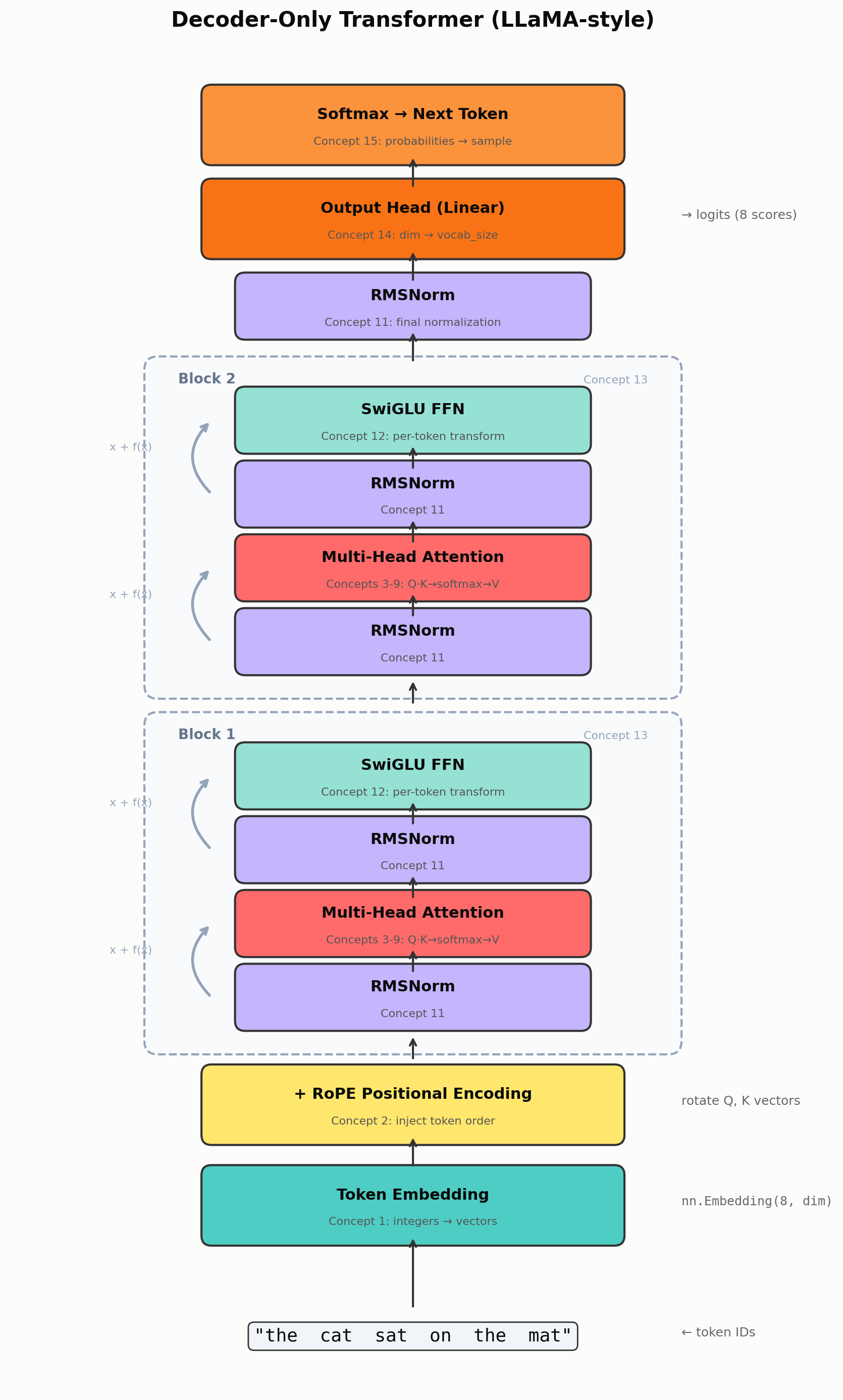
Let’s draw the transformer to see how data flows through it. This is the exact architecture implemented in src/ai_playground/models/transformer.py.

Show plotting code
def draw_transformer_architecture(n_layers=2):
    """Draw a diagram of the decoder-only transformer architecture."""
    fig, ax = plt.subplots(1, 1, figsize=(10, 14))
    ax.set_xlim(-1, 11)
    ax.set_ylim(-1, 20)
    ax.axis('off')
    ax.set_aspect('equal')

    # Colors for each concept
    C = {
        'embed': '#4ECDC4',    # teal
        'rope': '#FFE66D',     # yellow
        'attn': '#FF6B6B',     # red
        'ffn': '#95E1D3',      # light green
        'norm': '#C4B5FD',     # purple
        'residual': '#94A3B8', # gray
        'output': '#F97316',   # orange
        'softmax': '#FB923C',  # light orange
    }

    def box(x, y, w, h, label, color, sublabel=None, fontsize=11):
        rect = mpatches.FancyBboxPatch((x, y), w, h, boxstyle='round,pad=0.15',
                                        facecolor=color, edgecolor='#333', linewidth=1.5)
        ax.add_patch(rect)
        ax.text(x + w/2, y + h/2 + (0.15 if sublabel else 0), label,
                ha='center', va='center', fontsize=fontsize, fontweight='bold')
        if sublabel:
            ax.text(x + w/2, y + h/2 - 0.25, sublabel,
                    ha='center', va='center', fontsize=8, color='#555')

    def arrow(x1, y1, x2, y2, color='#333'):
        ax.annotate('', xy=(x2, y2), xytext=(x1, y1),
                    arrowprops=dict(arrowstyle='->', color=color, lw=1.5))

    # --- Input tokens ---
    y = 0
    ax.text(5, y, '"the  cat  sat  on  the  mat"', ha='center', va='center',
            fontsize=13, fontfamily='monospace',
            bbox=dict(boxstyle='round,pad=0.3', facecolor='#F1F5F9', edgecolor='#333'))
    ax.text(9, y, '← token IDs', ha='left', fontsize=9, color='#666')

    # --- Embedding ---
    y = 1.5
    arrow(5, 0.4, 5, y)
    box(2, y, 6, 0.9, 'Token Embedding', C['embed'], 'Concept 1: integers β†’ vectors')
    ax.text(9, y + 0.45, f'nn.Embedding({len(VOCAB)}, dim)', ha='left', fontsize=9,
            color='#666', fontfamily='monospace')

    # --- RoPE ---
    y = 3.0
    arrow(5, 2.5, 5, y)
    box(2, y, 6, 0.9, '+ RoPE Positional Encoding', C['rope'], 'Concept 2: inject token order')
    ax.text(9, y + 0.45, 'rotate Q, K vectors', ha='left', fontsize=9, color='#666')

    # --- Transformer blocks ---
    block_start = 4.5
    block_h = 4.5
    for i in range(n_layers):
        by = block_start + i * (block_h + 0.8)
        arrow(5, by - 0.4, 5, by)

        # Block border
        block_rect = mpatches.FancyBboxPatch((1.2, by - 0.1), 7.6, block_h + 0.2,
            boxstyle='round,pad=0.2', facecolor='#F8FAFC', edgecolor='#94A3B8',
            linewidth=1.5, linestyle='--')
        ax.add_patch(block_rect)
        ax.text(1.5, by + block_h - 0.1, f'Block {i+1}', fontsize=10,
                fontweight='bold', color='#64748B')
        ax.text(8.5, by + block_h - 0.1, 'Concept 13', fontsize=8, color='#94A3B8', ha='right')

        # RMSNorm
        ny1 = by + 0.2
        box(2.5, ny1, 5, 0.7, 'RMSNorm', C['norm'], 'Concept 11')

        # Attention
        ay = ny1 + 1.1
        arrow(5, ny1 + 0.7, 5, ay)
        box(2.5, ay, 5, 0.7, 'Multi-Head Attention', C['attn'], 'Concepts 3-9: Q·K→softmax→V')

        # Residual arrow for attention
        ax.annotate('', xy=(2.0, ay + 0.35), xytext=(2.0, ny1 + 0.35),
                    arrowprops=dict(arrowstyle='->', color=C['residual'], lw=2,
                                    connectionstyle='arc3,rad=-0.5'))
        ax.text(0.8, ay - 0.1, 'x + f(x)', fontsize=8, color=C['residual'], ha='center')

        # RMSNorm 2
        ny2 = ay + 1.1
        arrow(5, ay + 0.7, 5, ny2)
        box(2.5, ny2, 5, 0.7, 'RMSNorm', C['norm'], 'Concept 11')

        # FFN
        fy = ny2 + 1.1
        arrow(5, ny2 + 0.7, 5, fy)
        box(2.5, fy, 5, 0.7, 'SwiGLU FFN', C['ffn'], 'Concept 12: per-token transform')

        # Residual arrow for FFN
        ax.annotate('', xy=(2.0, fy + 0.35), xytext=(2.0, ny2 + 0.35),
                    arrowprops=dict(arrowstyle='->', color=C['residual'], lw=2,
                                    connectionstyle='arc3,rad=-0.5'))
        ax.text(0.8, fy - 0.1, 'x + f(x)', fontsize=8, color=C['residual'], ha='center')

    # --- Final norm ---
    ny = block_start + n_layers * (block_h + 0.8) - 0.1
    arrow(5, ny - 0.5, 5, ny)
    box(2.5, ny, 5, 0.7, 'RMSNorm', C['norm'], 'Concept 11: final normalization')

    # --- Output head ---
    oy = ny + 1.2
    arrow(5, ny + 0.7, 5, oy)
    box(2, oy, 6, 0.9, 'Output Head (Linear)', C['output'], 'Concept 14: dim β†’ vocab_size')
    ax.text(9, oy + 0.45, f'β†’ logits ({len(VOCAB)} scores)', ha='left', fontsize=9, color='#666')

    # --- Softmax ---
    sy = oy + 1.4
    arrow(5, oy + 0.9, 5, sy)
    box(2, sy, 6, 0.9, 'Softmax β†’ Next Token', C['softmax'], 'Concept 15: probabilities β†’ sample')

    ax.set_ylim(-0.8, sy + 1.6)
    ax.set_title('Decoder-Only Transformer (LLaMA-style)', fontsize=15, fontweight='bold', pad=15)

    plt.tight_layout()
    plt.show()

draw_transformer_architecture(n_layers=2)

2b. Understanding the Building Blocks

The architecture diagram above shows several components that deserve explanation before we start training. Each one solves a specific problem.

RMSNorm (the purple boxes)

Problem: As vectors flow through many layers, their magnitudes can grow or shrink uncontrollably. A vector that was [0.1, 0.2, 0.3] might become [500, 1000, 1500] after a few layers. This makes training unstable.

Solution: Normalize each vector to have unit RMS (root mean square). Divide by the vector’s average magnitude, then scale by a learned weight:

rms = sqrt(mean(xΒ²))
output = (x / rms) * weight

That’s it. Standard LayerNorm also subtracts the mean (centering), but Zhang & Sennrich (2019) showed the centering is unnecessary β€” removing it makes RMSNorm ~10-15% faster with no quality loss. Used in LLaMA, Mistral, Gemma, and most modern LLMs.

Implementation: src/ai_playground/models/layers.py β†’ RMSNorm Paper: Root Mean Square Layer Normalization See also: docs/PAPERS.md Β§ Normalization & Activations


SwiGLU FFN (the green boxes)

Problem: Attention lets tokens talk to each other, but it’s a linear operation (weighted average). The model also needs a nonlinear transformation applied to each token independently β€” this is where the model stores β€œknowledge” (facts, patterns, associations) in its weight matrices.

Solution: A feed-forward network (FFN) with a gated activation:

gate  = swish(x @ W_gate)     ← "how much to let through" (0 to 1-ish)
value = x @ W_up              ← "what to let through"
output = (gate * value) @ W_down

The swish function (= x Γ— sigmoid(x)) is a smooth version of ReLU. The gating mechanism (multiply gate Γ— value) lets the network learn to selectively activate different dimensions β€” like an if/else in the vector space.

Standard FFN uses 2 weight matrices. SwiGLU uses 3 (gate, up, down), but the hidden dimension is reduced by 2/3, so total parameters are similar while performance is consistently better.

Implementation: src/ai_playground/models/layers.py β†’ SwiGLU Paper: GLU Variants Improve Transformer (Shazeer, 2020) See also: docs/PAPERS.md Β§ Normalization & Activations


Why Softmax? (the orange boxes)

Problem: The model’s output is a vector of raw scores (logits) β€” one per vocabulary token. We need to convert these into probabilities that sum to 1 so we can sample the next token.

Why not just divide by the sum? Logits can be negative, and we want the highest score to get the most probability, with an exponential preference:

softmax(x_i) = exp(x_i) / sum(exp(x_j))
  • A score of 5.0 vs 3.0: softmax gives ~88% vs ~12% (strong preference)
  • A score of 1.0 vs 0.9: softmax gives ~52% vs ~48% (near-uniform)

The exponential amplifies differences β€” the model can be confidently decisive (one token dominates) or express genuine uncertainty (several tokens are plausible).

Softmax also appears inside attention (concept 6): after computing QΒ·K scores, softmax converts them to attention weights that sum to 1 for each query position. Same logic β€” we want a probability distribution over which tokens to attend to.

Reference: β€œAttention Is All You Need” Β§3.2.1


The AdamW Optimizer (used in training below)

Problem: Gradient descent says β€œmove parameters opposite to the gradient.” But how far? And what if gradients are noisy (different every batch)?

Solution: AdamW tracks two running averages for each parameter:

  1. Momentum (m): smoothed gradient direction β€” filters out noise, like a rolling average. If gradients consistently point left, momentum builds up and we take bigger steps left.

  2. Velocity (v): smoothed gradient magnitude β€” tells us how β€œsteep” the landscape is around this parameter. Parameters with large gradients get smaller effective learning rates (careful steps), and vice versa.

The update: ΞΈ = ΞΈ - lr Γ— momentum / sqrt(velocity)

The β€œW” in AdamW: weight decay is applied directly to parameters (ΞΈ = ΞΈ Γ— (1 - lr Γ— Ξ»)) rather than through the gradient. This simple fix, decoupling weight decay from the adaptive learning rate, meaningfully improves training.

Implementation: src/ai_playground/training/optimizers.py β†’ AdamWFromScratch For the full step-by-step build: notebooks/02_training_optimization/04_adamw_from_scratch.ipynb Paper: Decoupled Weight Decay Regularization (Loshchilov & Hutter, 2019) See also: docs/PAPERS.md Β§ Training Optimization

Code
# === RMSNorm in action ===
from ai_playground.models.layers import RMSNorm

x = torch.tensor([[3.0, 1.0, 4.0, 1.0, 5.0]])  # a vector with varying magnitudes
norm = RMSNorm(5)

with torch.no_grad():
    x_normed = norm(x)

rms = x.pow(2).mean().sqrt()
print('=== RMSNorm ===')
print(f'Input:      {x[0].tolist()}  (RMS = {rms:.2f})')
print(f'Normalized: {[round(v, 4) for v in x_normed[0].tolist()]}')
print(f'After norm, RMS \u2248 1.0 \u2014 magnitudes are controlled.\n')

# === SwiGLU FFN in action ===
from ai_playground.models.layers import SwiGLU

ffn = SwiGLU(dim=8, hidden_dim=16)
x_ffn = torch.randn(1, 3, 8)  # (batch=1, seq=3, dim=8)

with torch.no_grad():
    y_ffn = ffn(x_ffn)

print('=== SwiGLU FFN ===')
print(f'Input shape:  {list(x_ffn.shape)}  (batch, seq, dim)')
print(f'Output shape: {list(y_ffn.shape)}  (same \u2014 FFN transforms each token independently)')
print(f'Hidden dim:   16 (expanded from 8 for more expressive intermediate repr)')
print(f'Num params:   {sum(p.numel() for p in ffn.parameters())}  (3 matrices: gate, up, down)\n')

# === Softmax in action ===
print('=== Why Softmax? ===')
logits = torch.tensor([5.0, 3.0, 1.0, -1.0, -3.0])
probs = F.softmax(logits, dim=-1)
print(f'Raw logits:     {logits.tolist()}')
print(f'Softmax probs:  {[f"{p:.1%}" for p in probs.tolist()]}')
print(f'Sum of probs:   {probs.sum().item():.4f}  (always 1.0)')
print(f'Highest logit (5.0) gets {probs[0]:.0%} of probability \u2014 exponential amplifies differences.\n')

# Temperature effect (used in generation)
print('Temperature controls sharpness:')
for temp in [0.5, 1.0, 2.0]:
    p = F.softmax(logits / temp, dim=-1)
    label = "sharper" if temp < 1 else "flatter" if temp > 1 else "default"
    print(f'  temp={temp}: {[f"{v:.1%}" for v in p.tolist()]}  ({label})')

print('\nLow temperature \u2192 more confident. High temperature \u2192 more random.')
=== RMSNorm ===
Input:      [3.0, 1.0, 4.0, 1.0, 5.0]  (RMS = 3.22)
Normalized: [0.9303, 0.3101, 1.2403, 0.3101, 1.5504]
After norm, RMS β‰ˆ 1.0 β€” magnitudes are controlled.

=== SwiGLU FFN ===
Input shape:  [1, 3, 8]  (batch, seq, dim)
Output shape: [1, 3, 8]  (same β€” FFN transforms each token independently)
Hidden dim:   16 (expanded from 8 for more expressive intermediate repr)
Num params:   384  (3 matrices: gate, up, down)

=== Why Softmax? ===
Raw logits:     [5.0, 3.0, 1.0, -1.0, -3.0]
Softmax probs:  ['86.5%', '11.7%', '1.6%', '0.2%', '0.0%']
Sum of probs:   1.0000  (always 1.0)
Highest logit (5.0) gets 86% of probability β€” exponential amplifies differences.

Temperature controls sharpness:
  temp=0.5: ['98.2%', '1.8%', '0.0%', '0.0%', '0.0%']  (sharper)
  temp=1.0: ['86.5%', '11.7%', '1.6%', '0.2%', '0.0%']  (default)
  temp=2.0: ['63.6%', '23.4%', '8.6%', '3.2%', '1.2%']  (flatter)

Low temperature β†’ more confident. High temperature β†’ more random.

3. Build Our Tiny Model

A 2-layer transformer with dim=32. Small enough to watch every detail, but uses the exact same code as the larger configs.

Code
# Tiny config β€” same TransformerConfig, just very small numbers
config = TransformerConfig(
    vocab_size=len(VOCAB),   # 8 tokens
    dim=32,                  # 32-dimensional vectors
    n_layers=2,              # 2 transformer blocks
    n_heads=4,               # 4 attention heads
    n_kv_heads=2,            # GQA: 2 KV heads shared by 4 Q heads
    max_seq_len=16,
    ffn_dim_multiplier=2.0,
)

model = Transformer(config).to(device)
n_params = sum(p.numel() for p in model.parameters())
print(f'Model: {config.n_layers} layers, dim={config.dim}, {n_params:,} parameters')
print(f'Vocab: {len(VOCAB)} tokens')
print(f'Head dim: {config.head_dim}, KV heads: {config.kv_heads}')
Model: 2 layers, dim=32, 19,104 parameters
Vocab: 8 tokens
Head dim: 8, KV heads: 2

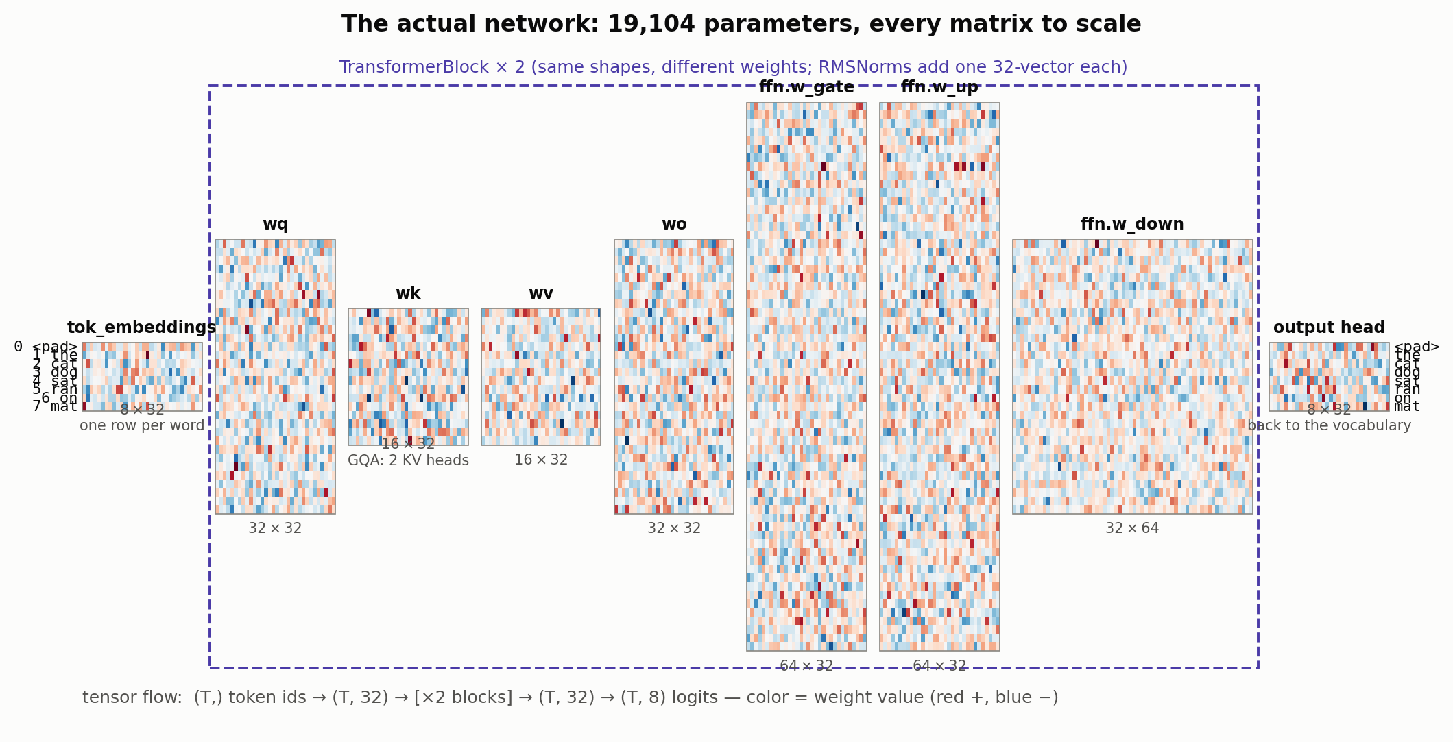
The actual network, to scale

Diagrams of transformers usually show boxes. This is the real thing: every weight matrix of the model we just built, drawn to scale (one square per weight), with the 8-word vocabulary visible at both ends β€” each word owns one 32-dim row of the embedding table, and the output head maps back to exactly those 8 words. Weights are at initialization here; Β§5 trains them.

Show diagram code
def draw_actual_network(model):
    """Every weight matrix, to scale, labeled with its true shape."""
    fig, ax = plt.subplots(figsize=(13, 6.5))
    ax.axis('off'); ax.grid(False)
    MID, GAP = 36, 3.5

    def put(w, x, name, note=None):
        """imshow weight (out, in) as an in-wide x out-tall block; return next x."""
        h, wid = w.shape
        y0 = MID - h / 2
        lim = float(w.abs().max())
        ax.imshow(w.detach(), extent=[x, x + wid, y0, y0 + h], cmap='RdBu_r',
                  vmin=-lim, vmax=lim, aspect='auto', interpolation='nearest')
        ax.add_patch(plt.Rectangle((x, y0), wid, h, fill=False, ec='#898781', lw=0.6))
        ax.text(x + wid / 2, y0 + h + 1.2, name, ha='center', fontsize=8.5,
                fontweight='semibold')
        ax.text(x + wid / 2, y0 - 2.2, f'{h}\u2009\u00d7\u2009{wid}' + (f'\n{note}' if note else ''),
                ha='center', fontsize=7.5, color='#52514e')
        return x + wid + GAP

    # vocabulary -> embedding rows
    E = model.tok_embeddings.weight            # (8, 32)
    x = 8.5
    y0 = MID - E.shape[0] / 2
    for i, wrd in enumerate(VOCAB):
        ax.text(x - 1.2, y0 + E.shape[0] - i - 0.5, f'{i} {wrd}',
                ha='right', va='center', fontsize=8, family='monospace')
    x = put(E, x, 'tok_embeddings', 'one row per word')

    # one transformer block, expanded (both blocks share these shapes)
    blk = model.layers[0]
    x_block0 = x
    x = put(blk.attention.wq.weight, x, 'wq')
    x = put(blk.attention.wk.weight, x, 'wk', 'GQA: 2 KV heads')
    x = put(blk.attention.wv.weight, x, 'wv')
    x = put(blk.attention.wo.weight, x, 'wo')
    for name, p in blk.feed_forward.named_parameters():
        if p.ndim == 2:
            x = put(p, x, f'ffn.{name.split(".")[0]}')
    ax.add_patch(plt.Rectangle((x_block0 - 1.5, MID - 34), x - x_block0 - GAP + 3, 68,
                               fill=False, ec='#4a3aa7', lw=1.4, ls='--'))
    ax.text((x_block0 + x - GAP) / 2, MID + 35.5,
            f'TransformerBlock \u00d7 {config.n_layers} (same shapes, different weights; '
            'RMSNorms add one 32-vector each)', ha='center', fontsize=9, color='#4a3aa7')

    # output head -> the same 8 words as logits
    O = model.output.weight                    # (8, 32)
    x_out = x + 1
    x = put(O, x_out, 'output head', 'back to the vocabulary')
    y0 = MID - O.shape[0] / 2
    for i, wrd in enumerate(VOCAB):
        ax.text(x - GAP + 1.2, y0 + O.shape[0] - i - 0.5, f'{wrd}',
                ha='left', va='center', fontsize=8, family='monospace')

    ax.text(8.5, MID - 38, 'tensor flow:  (T,) token ids \u2192 (T, 32) \u2192 '
            f'[\u00d7{config.n_layers} blocks] \u2192 (T, 32) \u2192 (T, 8) logits '
            '\u2014 color = weight value (red +, blue \u2212)',
            fontsize=9, color='#52514e')
    ax.set_xlim(0, x + 8); ax.set_ylim(MID - 41, MID + 39)
    ax.set_title(f'The actual network: {sum(p.numel() for p in model.parameters()):,} '
                 'parameters, every matrix to scale', fontsize=12)
    plt.show()

draw_actual_network(model)
/var/folders/gm/lny259x17rjchmw201s4sfh80000gn/T/ipykernel_78503/977902726.py:13: UserWarning: Converting a tensor with requires_grad=True to a scalar may lead to unexpected behavior.
Consider using tensor.detach() first. (Triggered internally at /Users/runner/work/pytorch/pytorch/pytorch/torch/csrc/autograd/generated/python_variable_methods.cpp:837.)
  lim = float(w.abs().max())

4. Trace a Single Forward Pass

Let’s follow the sentence "the cat sat on the mat" through the model and see what comes out at each stage.

Code
# Tokenize and prepare input
sentence = 'the cat sat on the mat'
tokens = tokenize(sentence)
token_ids = torch.tensor([tokens], device=device)  # (1, 6)

print(f'Input:     "{sentence}"')
print(f'Token IDs: {tokens}')
print(f'Shape:     {token_ids.shape}  (batch=1, seq_len=6)\n')

# --- Concept 1: Embedding ---
with torch.no_grad():
    embeddings = model.tok_embeddings(token_ids)
print(f'After embedding (concept 1):')
print(f'  Shape: {embeddings.shape}  (batch, seq_len, dim={config.dim})')
print(f'  Each token is now a {config.dim}-dim vector')
print(f'  "the" β†’ [{embeddings[0, 0, :4].tolist()}  ...]')
print(f'  "cat" β†’ [{embeddings[0, 1, :4].tolist()}  ...]\n')

# --- Concept 2: Same word, different position ---
print(f'Same word "the" at position 0 vs position 4:')
print(f'  Position 0: [{embeddings[0, 0, :6].tolist()}  ...]')
print(f'  Position 4: [{embeddings[0, 4, :6].tolist()}  ...]')
print(f'  Before RoPE these are identical β€” RoPE rotates Q,K inside attention')
print(f'  to make the model aware of position.\n')

# --- Full forward pass β†’ logits ---
with torch.no_grad():
    logits = model(token_ids)  # (1, 6, vocab_size)
print(f'Output logits (concept 14):')
print(f'  Shape: {logits.shape}  (batch, seq_len, vocab_size={config.vocab_size})')
print(f'  Each position has {config.vocab_size} scores β€” one per vocabulary token\n')

# --- Concept 15: Softmax β†’ probabilities ---
probs = F.softmax(logits[0], dim=-1)  # (6, 8)

print('Predictions at each position (before training β€” random!):')
for i in range(len(tokens)):
    top_prob, top_id = probs[i].topk(3)
    preds = ', '.join(f'{id2tok[j.item()]}({p:.0%})' for p, j in zip(top_prob, top_id))
    target = id2tok[tokens[i+1]] if i+1 < len(tokens) else '(end)'
    print(f'  After "{id2tok[tokens[i]]}" β†’ predicts: {preds}   (should be: {target})')
Input:     "the cat sat on the mat"
Token IDs: [1, 2, 4, 6, 1, 7]
Shape:     torch.Size([1, 6])  (batch=1, seq_len=6)

After embedding (concept 1):
  Shape: torch.Size([1, 6, 32])  (batch, seq_len, dim=32)
  Each token is now a 32-dim vector
  "the" β†’ [[-0.0320155955851078, -0.009524675086140633, 0.0022061688359826803, -0.0008383149397559464]  ...]
  "cat" β†’ [[0.004457029979676008, 0.03946416452527046, -0.01665784791111946, 0.005129831377416849]  ...]

Same word "the" at position 0 vs position 4:
  Position 0: [[-0.0320155955851078, -0.009524675086140633, 0.0022061688359826803, -0.0008383149397559464, -0.006199481897056103, 0.001743849366903305]  ...]
  Position 4: [[-0.0320155955851078, -0.009524675086140633, 0.0022061688359826803, -0.0008383149397559464, -0.006199481897056103, 0.001743849366903305]  ...]
  Before RoPE these are identical β€” RoPE rotates Q,K inside attention
  to make the model aware of position.

Output logits (concept 14):
  Shape: torch.Size([1, 6, 8])  (batch, seq_len, vocab_size=8)
  Each position has 8 scores β€” one per vocabulary token

Predictions at each position (before training β€” random!):
  After "the" β†’ predicts: mat(14%), ran(14%), sat(13%)   (should be: cat)
  After "cat" β†’ predicts: on(15%), dog(13%), cat(13%)   (should be: sat)
  After "sat" β†’ predicts: sat(17%), on(13%), mat(13%)   (should be: on)
  After "on" β†’ predicts: on(14%), mat(13%), the(13%)   (should be: the)
  After "the" β†’ predicts: ran(14%), mat(14%), on(13%)   (should be: mat)
  After "mat" β†’ predicts: ran(16%), mat(13%), the(13%)   (should be: (end))

4b. Watch a matmul happen in 3D

Every arrow in the forward pass above is a matrix multiplication. The one that produces the logits is the easiest to see whole: the final hidden states h β€” shape (6, 32), one row per token of our sentence β€” multiply the output head W_out β€” shape (32, 8), one column per vocabulary token β€” giving the (6, 8) logits we just printed.

The interactive view below (mm, from the PyTorch blog post Inside the Matrix) renders this exact matmul as a 3D volume: the inputs are two faces of a box, the result is a third, and the animated sweep computes one rowΒ·column dot product per cell of the result. Drag to spin, two-finger swipe to zoom.

Things to try:

  • Follow one row of h (a token’s final 32-dim vector): it meets all 8 columns of W_out to produce that token’s 8 logit scores β€” the same scores softmax turned into next-token probabilities in Β§4.
  • In the mm panel (top right), set epilog to softmax and watch each row of logits become a probability distribution.
  • Open this preset for a preview of the next chapter’s star matmul: one attention head’s Q @ Kα΅€ ((6, 8) @ (8, 6), head_dim = 8 from our config) with the causal-softmax epilog softmax(tril(x/√k)) applied β€” the (6, 6) result is the attention-weight matrix.

(The embed needs WebGL and won’t render in Colab β€” open it full-screen instead.)

5. Training: Watch the Model Learn

Now let’s train for 200 steps and track: - Loss β€” how wrong the predictions are (lower = better) - Predictions β€” what the model thinks comes next - Accuracy β€” fraction of correct next-token predictions

The training objective is next-token prediction: given the cat sat, predict that on comes next. This is done at every position simultaneously.

Code
# Prepare training data: input = tokens[:-1], target = tokens[1:]
# "the cat sat on the mat" β†’ input: "the cat sat on the", target: "cat sat on the mat"
train_x = []
train_y = []
for s in sentences:
    ids = tokenize(s)
    train_x.append(ids[:-1])   # all tokens except last
    train_y.append(ids[1:])    # all tokens except first (shifted by 1)

train_x = torch.tensor(train_x, device=device)  # (4, 5)
train_y = torch.tensor(train_y, device=device)  # (4, 5)

print('Training data (next-token prediction):')
print(f'  Batch size: {train_x.shape[0]} sentences')
print(f'  Sequence length: {train_x.shape[1]} tokens\n')
for i in range(len(sentences)):
    inp = [id2tok[j.item()] for j in train_x[i]]
    tgt = [id2tok[j.item()] for j in train_y[i]]
    print(f'  Input:  {inp}')
    print(f'  Target: {tgt}\n')
Training data (next-token prediction):
  Batch size: 4 sentences
  Sequence length: 5 tokens

  Input:  ['the', 'cat', 'sat', 'on', 'the']
  Target: ['cat', 'sat', 'on', 'the', 'mat']

  Input:  ['the', 'dog', 'ran', 'on', 'the']
  Target: ['dog', 'ran', 'on', 'the', 'mat']

  Input:  ['the', 'cat', 'ran', 'on', 'the']
  Target: ['cat', 'ran', 'on', 'the', 'mat']

  Input:  ['the', 'dog', 'sat', 'on', 'the']
  Target: ['dog', 'sat', 'on', 'the', 'mat']
Code
# Training loop
# AdamW optimizer (https://arxiv.org/abs/1711.05101)
# See docs/PAPERS.md Β§ Training Optimization
optimizer = torch.optim.AdamW(model.parameters(), lr=3e-3, weight_decay=0.01)

n_steps = 200
log_every = 10
snapshot_steps = [0, 5, 20, 50, 100, 199]  # capture predictions at these steps

losses = []
accuracies = []
snapshots = []  # (step, predictions_per_position)

model.train()
for step in range(n_steps):
    logits = model(train_x)  # (4, 5, 8)
    loss = F.cross_entropy(logits.view(-1, config.vocab_size), train_y.view(-1))

    optimizer.zero_grad()
    loss.backward()
    optimizer.step()

    # Track metrics
    with torch.no_grad():
        preds = logits.argmax(dim=-1)  # (4, 5)
        acc = (preds == train_y).float().mean().item()
        losses.append(loss.item())
        accuracies.append(acc)

    # Snapshot predictions for visualization
    if step in snapshot_steps:
        with torch.no_grad():
            probs = F.softmax(logits[0], dim=-1)  # first sentence
            snap = []
            for i in range(train_x.shape[1]):
                top_p, top_i = probs[i].topk(3)
                snap.append([(id2tok[j.item()], p.item()) for p, j in zip(top_p, top_i)])
            snapshots.append((step, snap))

    if step % log_every == 0 or step == n_steps - 1:
        print(f'Step {step:3d} | loss: {loss.item():.4f} | accuracy: {acc:.0%}')

print(f'\nFinal loss: {losses[-1]:.4f}, Final accuracy: {accuracies[-1]:.0%}')
Step   0 | loss: 2.0613 | accuracy: 0%
Step  10 | loss: 1.1334 | accuracy: 80%
Step  20 | loss: 0.6645 | accuracy: 80%
Step  30 | loss: 0.4413 | accuracy: 80%
Step  40 | loss: 0.3564 | accuracy: 80%
Step  50 | loss: 0.3237 | accuracy: 80%
Step  60 | loss: 0.3089 | accuracy: 80%
Step  70 | loss: 0.3011 | accuracy: 80%
Step  80 | loss: 0.2964 | accuracy: 80%
Step  90 | loss: 0.2932 | accuracy: 80%
Step 100 | loss: 0.2908 | accuracy: 80%
Step 110 | loss: 0.2890 | accuracy: 80%
Step 120 | loss: 0.2875 | accuracy: 80%
Step 130 | loss: 0.2864 | accuracy: 80%
Step 140 | loss: 0.2854 | accuracy: 80%
Step 150 | loss: 0.2846 | accuracy: 80%
Step 160 | loss: 0.2839 | accuracy: 80%
Step 170 | loss: 0.2833 | accuracy: 80%
Step 180 | loss: 0.2827 | accuracy: 80%
Step 190 | loss: 0.2823 | accuracy: 80%
Step 199 | loss: 0.2819 | accuracy: 80%

Final loss: 0.2819, Final accuracy: 80%

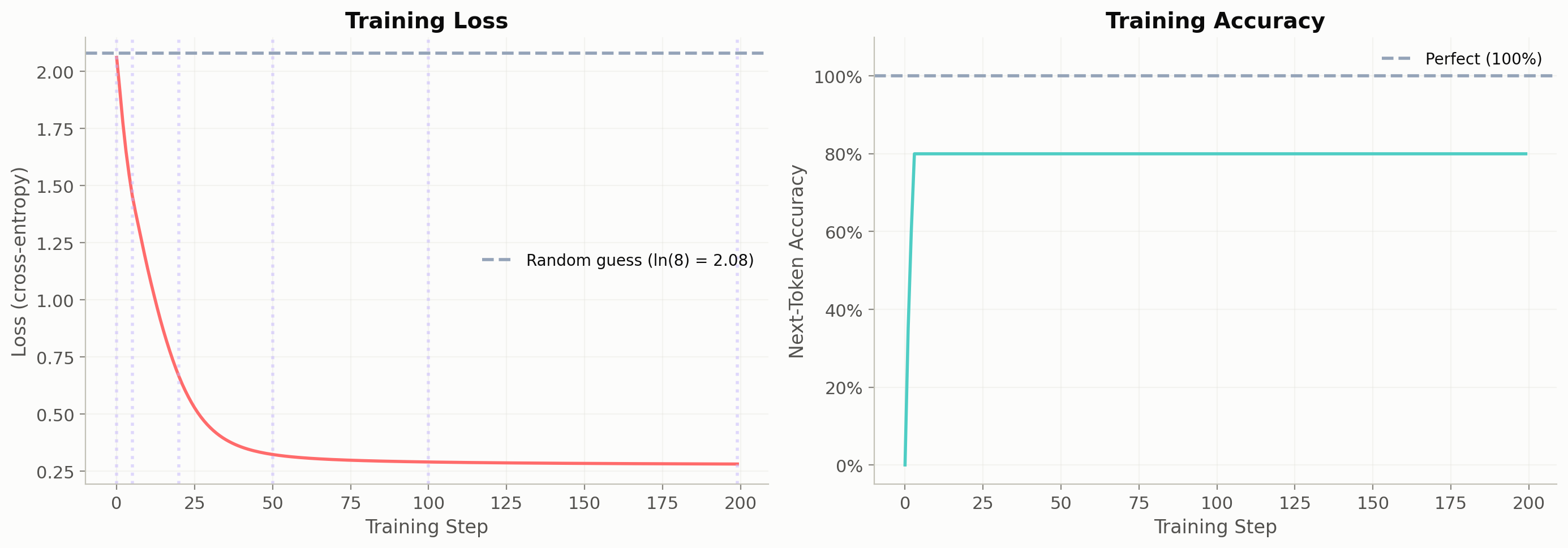
6. Loss & Accuracy Over Training

Loss measures how surprised the model is by the correct answer (cross-entropy). It starts high (random guessing over 8 tokens β†’ loss β‰ˆ ln(8) β‰ˆ 2.08) and drops as the model learns the patterns.

Code
fig, (ax1, ax2) = plt.subplots(1, 2, figsize=(14, 5))

# Loss curve
ax1.plot(losses, color='#FF6B6B', linewidth=2)
ax1.axhline(y=np.log(len(VOCAB)), color='#94A3B8', linestyle='--', label=f'Random guess (ln({len(VOCAB)}) = {np.log(len(VOCAB)):.2f})')
ax1.set_xlabel('Training Step', fontsize=12)
ax1.set_ylabel('Loss (cross-entropy)', fontsize=12)
ax1.set_title('Training Loss', fontsize=14, fontweight='bold')
ax1.legend(fontsize=10)
ax1.grid(True, alpha=0.3)

# Mark snapshot steps
for s, _ in snapshots:
    ax1.axvline(x=s, color='#C4B5FD', alpha=0.5, linestyle=':')

# Accuracy curve
ax2.plot(accuracies, color='#4ECDC4', linewidth=2)
ax2.axhline(y=1.0, color='#94A3B8', linestyle='--', label='Perfect (100%)')
ax2.set_xlabel('Training Step', fontsize=12)
ax2.set_ylabel('Next-Token Accuracy', fontsize=12)
ax2.set_title('Training Accuracy', fontsize=14, fontweight='bold')
ax2.set_ylim(-0.05, 1.1)
ax2.yaxis.set_major_formatter(plt.FuncFormatter(lambda y, _: f'{y:.0%}'))
ax2.legend(fontsize=10)
ax2.grid(True, alpha=0.3)

plt.tight_layout()
plt.show()

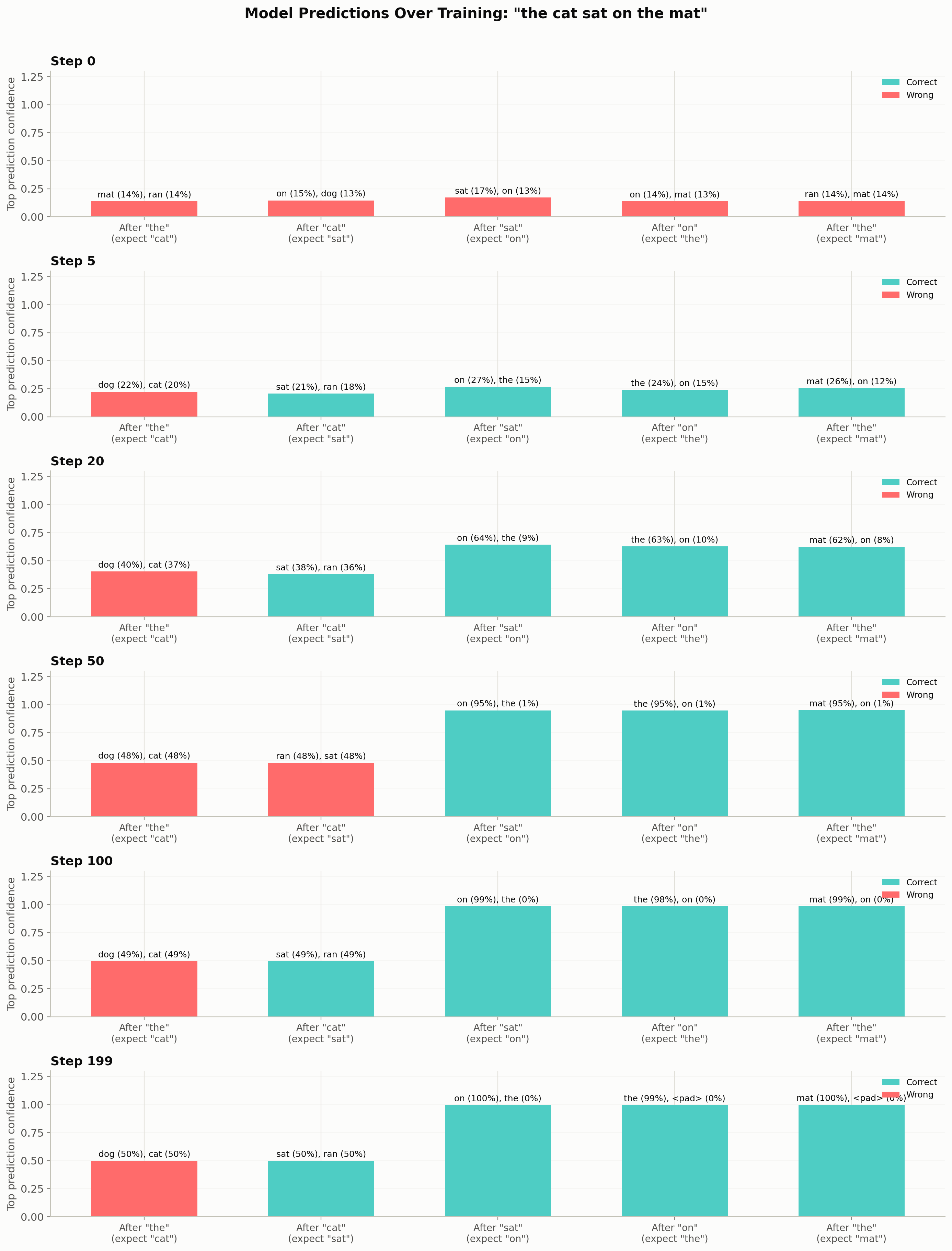
7. Predictions at Each Training Step

Watch the model go from random guessing to confident correct predictions. We trace the first sentence: "the cat sat on the mat".

Show plotting code
input_tokens = [id2tok[j.item()] for j in train_x[0]]
target_tokens = [id2tok[j.item()] for j in train_y[0]]

fig, axes = plt.subplots(len(snapshots), 1, figsize=(14, 3 * len(snapshots)))

for idx, (step, snap) in enumerate(snapshots):
    ax = axes[idx]
    positions = range(len(input_tokens))

    # Build heatmap data: (n_positions, vocab_size) but only show top predictions
    bars_correct = []
    bars_wrong = []
    labels = []

    for i, preds in enumerate(snap):
        target = target_tokens[i]
        top_word, top_prob = preds[0]
        correct = (top_word == target)
        bars_correct.append(top_prob if correct else 0)
        bars_wrong.append(top_prob if not correct else 0)
        pred_str = ', '.join(f'{w} ({p:.0%})' for w, p in preds[:2])
        labels.append(pred_str)

    x = np.arange(len(input_tokens))
    ax.bar(x, bars_correct, color='#4ECDC4', label='Correct', width=0.6)
    ax.bar(x, bars_wrong, color='#FF6B6B', label='Wrong', width=0.6)

    # Annotate
    for i, label in enumerate(labels):
        ax.text(i, max(bars_correct[i], bars_wrong[i]) + 0.02, label,
                ha='center', va='bottom', fontsize=9, rotation=0)

    ax.set_xticks(x)
    ax.set_xticklabels([f'After "{t}"\n(expect "{target_tokens[i]}")'
                        for i, t in enumerate(input_tokens)], fontsize=10)
    ax.set_ylim(0, 1.3)
    ax.set_ylabel('Top prediction confidence')
    ax.set_title(f'Step {step}', fontsize=13, fontweight='bold', loc='left')
    ax.legend(loc='upper right', fontsize=9)
    ax.grid(True, alpha=0.2, axis='y')

plt.suptitle('Model Predictions Over Training: "the cat sat on the mat"',
             fontsize=15, fontweight='bold', y=1.01)
plt.tight_layout()
plt.show()

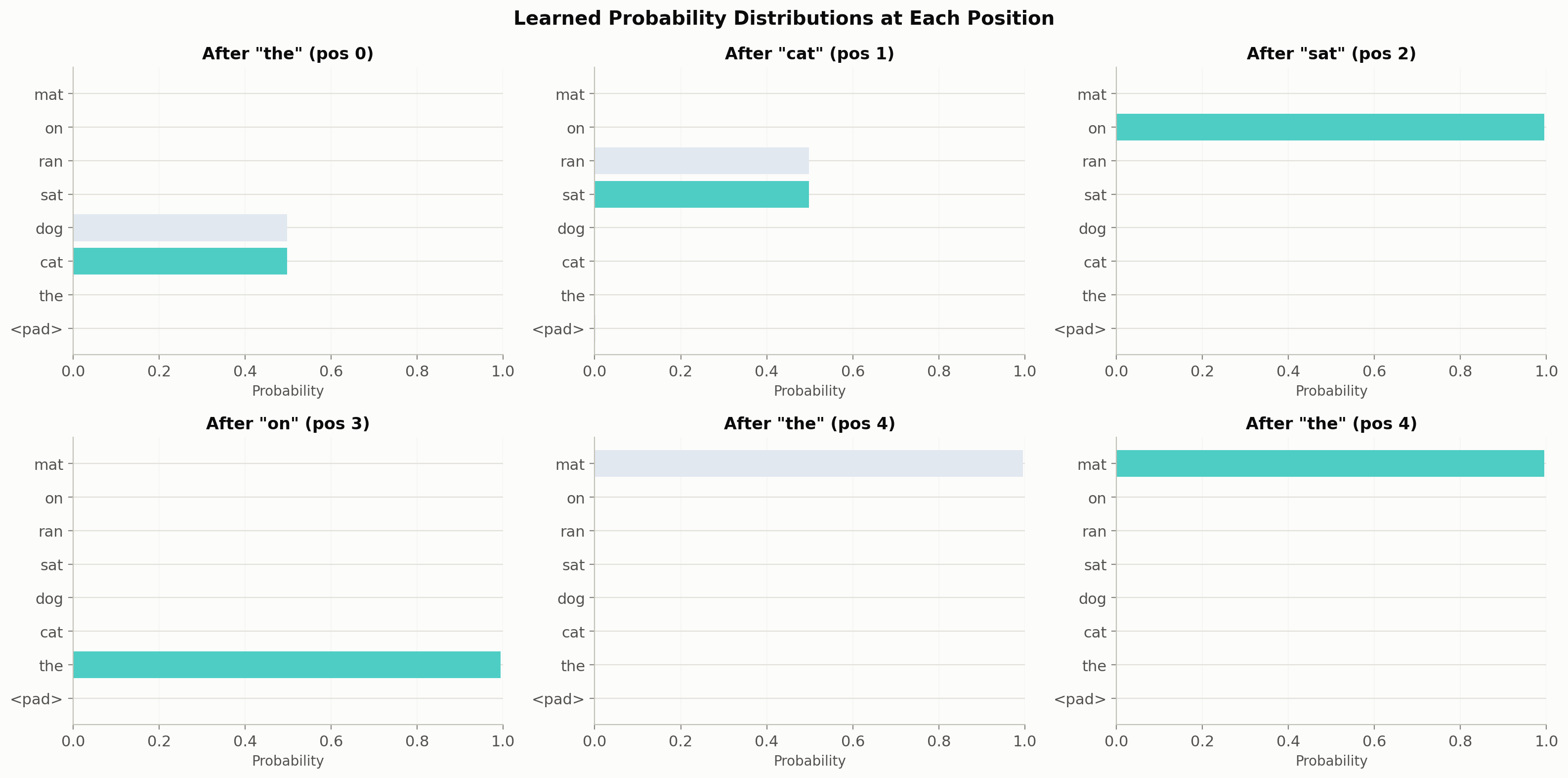
8. What Did the Model Learn?

Let’s look at the final probability distribution at each position. A well-trained model should be confident about deterministic positions (the β†’ always followed by cat or dog) and uncertain where multiple options are valid.

Show plotting code
model.eval()

fig, axes = plt.subplots(2, 3, figsize=(16, 8))
axes = axes.flatten()

sentence = 'the cat sat on the'
tokens_viz = tokenize(sentence)
token_ids_viz = torch.tensor([tokens_viz], device=device)

with torch.no_grad():
    logits_viz = model(token_ids_viz)
    probs_viz = F.softmax(logits_viz[0], dim=-1)

for i, ax in enumerate(axes[:len(tokens_viz)]):
    p = probs_viz[i].cpu().numpy()
    colors = ['#4ECDC4' if j == (tokens_viz[i+1] if i+1 < len(tokens_viz) else -1)
              else '#E2E8F0' for j in range(len(VOCAB))]
    ax.barh(range(len(VOCAB)), p, color=colors)
    ax.set_yticks(range(len(VOCAB)))
    ax.set_yticklabels(VOCAB, fontsize=11)
    ax.set_xlim(0, 1)
    ax.set_xlabel('Probability', fontsize=10)
    ax.set_title(f'After "{id2tok[tokens_viz[i]]}" (pos {i})', fontsize=12, fontweight='bold')
    ax.grid(True, alpha=0.2, axis='x')

# Last subplot: show prediction for the full sequence
ax = axes[len(tokens_viz)]
p = probs_viz[-1].cpu().numpy()
colors = ['#4ECDC4' if VOCAB[j] == 'mat' else '#E2E8F0' for j in range(len(VOCAB))]
ax.barh(range(len(VOCAB)), p, color=colors)
ax.set_yticks(range(len(VOCAB)))
ax.set_yticklabels(VOCAB, fontsize=11)
ax.set_xlim(0, 1)
ax.set_xlabel('Probability', fontsize=10)
ax.set_title(f'After "the" (pos {len(tokens_viz)-1})', fontsize=12, fontweight='bold')
ax.grid(True, alpha=0.2, axis='x')

plt.suptitle('Learned Probability Distributions at Each Position',
             fontsize=14, fontweight='bold')
plt.tight_layout()
plt.show()

print('Green = correct next token.')
print('Notice: after "the" the model may assign probability to both "cat" and "dog"')
print('because both are valid continuations in our training data.')

Green = correct next token.
Notice: after "the" the model may assign probability to both "cat" and "dog"
because both are valid continuations in our training data.

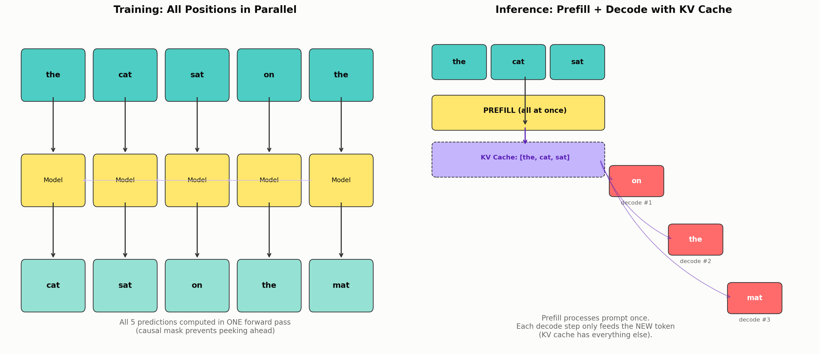
8b. Training vs Inference: Two Different Modes

The same model is used in two very different ways. Understanding the difference is key to understanding why the KV cache exists.

Training Mode

During training, the model sees the entire sequence at once:

Input:  [the, cat, sat, on, the]     ← all 5 tokens, single forward pass
Target: [cat, sat, on, the, mat]     ← predict next token at every position
  • All positions computed in parallel β€” the causal mask ensures each position can only attend to earlier positions, but the GPU processes them all simultaneously.
  • No KV cache needed β€” we process the full sequence once, compute loss, backpropagate.
  • Efficient: one forward + one backward pass per batch.

Inference Mode (Generation)

During generation, the model produces one token at a time:

Step 1 (prefill):  [the, cat, sat, on, the] β†’ model β†’ predict "mat"
                    └─ process entire prompt, cache all K,V

Step 2 (decode):   [mat] β†’ model (reuses cached K,V) β†’ predict next
                    └─ only the NEW token goes through the model

Step 3 (decode):   [next] β†’ model (extends cache) β†’ predict next
                    ...
  • Prefill: process the full prompt in one pass (like training). This populates the KV cache β€” each attention layer stores its Key and Value tensors.
  • Decode: only feed the single new token. Inside attention, its Query attends to all cached Keys/Values, but we don’t recompute K,V for old tokens.
  • Without KV cache: every decode step would reprocess all previous tokens β†’ O(nΒ²) total.
  • With KV cache: each decode step only computes the new token β†’ O(n) per step.

The KV Cache

Each attention layer stores two tensors per token: - K (Key): what this token β€œadvertises” for matching - V (Value): what information this token carries

For a model with n_layers=2, n_kv_heads=2, head_dim=8:

Cache per token = 2 (K+V) Γ— 2 (layers) Γ— 2 (kv_heads) Γ— 8 (head_dim) = 64 values
For 1024 tokens = 64 Γ— 1024 = 65,536 values Γ— 2 bytes (FP16) = 128 KB

For real models this adds up fast β€” see the KV cache table in notebooks/01_transformer_internals/01_attention_mechanisms.ipynb for LLaMA-scale numbers.

Reference: src/ai_playground/inference/generate.py Β· PagedAttention (vLLM) See also: docs/PAPERS.md Β§ Inference Optimization

Show plotting code
# === Visualize Training vs Inference ===
fig, (ax1, ax2) = plt.subplots(1, 2, figsize=(16, 7))

# --- Left: Training (parallel) ---
ax = ax1
tokens_train = ['the', 'cat', 'sat', 'on', 'the']
targets_train = ['cat', 'sat', 'on', 'the', 'mat']
n = len(tokens_train)

for i in range(n):
    # Input token
    ax.add_patch(mpatches.FancyBboxPatch((i * 1.8, 4), 1.4, 0.8,
        boxstyle='round,pad=0.1', facecolor='#4ECDC4', edgecolor='#333'))
    ax.text(i * 1.8 + 0.7, 4.4, tokens_train[i], ha='center', va='center',
            fontsize=11, fontweight='bold')
    # Arrow down
    ax.annotate('', xy=(i * 1.8 + 0.7, 2.9), xytext=(i * 1.8 + 0.7, 4.0),
                arrowprops=dict(arrowstyle='->', color='#333', lw=1.5))
    # Model box
    ax.add_patch(mpatches.FancyBboxPatch((i * 1.8, 2.0), 1.4, 0.8,
        boxstyle='round,pad=0.1', facecolor='#FFE66D', edgecolor='#333'))
    ax.text(i * 1.8 + 0.7, 2.4, 'Model', ha='center', va='center', fontsize=9)
    # Arrow down
    ax.annotate('', xy=(i * 1.8 + 0.7, 0.9), xytext=(i * 1.8 + 0.7, 2.0),
                arrowprops=dict(arrowstyle='->', color='#333', lw=1.5))
    # Prediction
    ax.add_patch(mpatches.FancyBboxPatch((i * 1.8, 0.0), 1.4, 0.8,
        boxstyle='round,pad=0.1', facecolor='#95E1D3', edgecolor='#333'))
    ax.text(i * 1.8 + 0.7, 0.4, targets_train[i], ha='center', va='center',
            fontsize=11, fontweight='bold')

# Causal mask arrows (each token attends to previous)
for i in range(1, n):
    for j in range(i):
        ax.annotate('', xy=(j * 1.8 + 1.4, 2.4), xytext=(i * 1.8, 2.4),
                    arrowprops=dict(arrowstyle='->', color='#C4B5FD', lw=0.8, alpha=0.4))

ax.set_xlim(-0.5, n * 1.8 + 0.5)
ax.set_ylim(-0.8, 5.5)
ax.axis('off')
ax.set_title('Training: All Positions in Parallel', fontsize=14, fontweight='bold')
ax.text(n * 0.9, -0.5, 'All 5 predictions computed in ONE forward pass\n(causal mask prevents peeking ahead)',
        ha='center', fontsize=10, color='#666')

# --- Right: Inference (sequential with KV cache) ---
ax = ax2
prompt = ['the', 'cat', 'sat']
generated = ['on', 'the', 'mat']
all_toks = prompt + generated

# Prefill phase
for i, tok in enumerate(prompt):
    color = '#4ECDC4'
    ax.add_patch(mpatches.FancyBboxPatch((i * 1.3, 5.5), 1.0, 0.7,
        boxstyle='round,pad=0.1', facecolor=color, edgecolor='#333'))
    ax.text(i * 1.3 + 0.5, 5.85, tok, ha='center', va='center', fontsize=10, fontweight='bold')

ax.add_patch(mpatches.FancyBboxPatch((0, 4.2), len(prompt) * 1.3 - 0.3, 0.7,
    boxstyle='round,pad=0.1', facecolor='#FFE66D', edgecolor='#333'))
ax.text(len(prompt) * 0.65, 4.55, 'PREFILL (all at once)', ha='center', fontsize=10, fontweight='bold')
ax.annotate('', xy=(len(prompt) * 0.65, 4.2), xytext=(len(prompt) * 0.65, 5.5),
            arrowprops=dict(arrowstyle='->', color='#333', lw=1.5))

# KV Cache box
cache_y = 3.0
ax.add_patch(mpatches.FancyBboxPatch((0, cache_y), len(prompt) * 1.3 - 0.3, 0.7,
    boxstyle='round,pad=0.1', facecolor='#C4B5FD', edgecolor='#333', linestyle='--'))
ax.text(len(prompt) * 0.65, cache_y + 0.35, 'KV Cache: [the, cat, sat]',
        ha='center', fontsize=9, fontweight='bold', color='#5B21B6')
ax.annotate('', xy=(len(prompt) * 0.65, cache_y + 0.7), xytext=(len(prompt) * 0.65, 4.2),
            arrowprops=dict(arrowstyle='->', color='#5B21B6', lw=1.5))

# Decode steps
for step, tok in enumerate(generated):
    y_base = 1.8 - step * 1.5
    x_new = (len(prompt) + step) * 1.3

    # New token input
    ax.add_patch(mpatches.FancyBboxPatch((x_new, y_base + 0.7), 1.0, 0.6,
        boxstyle='round,pad=0.1', facecolor='#FF6B6B', edgecolor='#333'))
    ax.text(x_new + 0.5, y_base + 1.0, tok, ha='center', va='center',
            fontsize=10, fontweight='bold', color='white')

    # Arrow from cache to new token
    ax.annotate('', xy=(x_new, y_base + 1.0),
                xytext=(len(prompt) * 1.3 - 0.3, cache_y + 0.35),
                arrowprops=dict(arrowstyle='->', color='#5B21B6', lw=1, alpha=0.5,
                                connectionstyle='arc3,rad=0.2'))

    # Label
    cached = prompt + generated[:step]
    ax.text(x_new + 0.5, y_base + 0.4, f'decode #{step+1}',
            ha='center', fontsize=8, color='#666')

ax.set_xlim(-0.5, (len(prompt) + len(generated)) * 1.3 + 0.5)
ax.set_ylim(-1.5, 7.0)
ax.axis('off')
ax.set_title('Inference: Prefill + Decode with KV Cache', fontsize=14, fontweight='bold')
ax.text(3.5, -1.2, 'Prefill processes prompt once.\nEach decode step only feeds the NEW token\n(KV cache has everything else).',
        ha='center', fontsize=10, color='#666')

plt.tight_layout()
plt.show()

# === Show cache growth ===
print('=== KV Cache Growth During Generation ===')
print(f'Model: {config.n_layers} layers, {config.kv_heads} KV heads, head_dim={config.head_dim}')
print(f'Cache per token: 2 (K+V) \u00d7 {config.n_layers} layers \u00d7 {config.kv_heads} heads \u00d7 {config.head_dim} dim = {2 * config.n_layers * config.kv_heads * config.head_dim} values\n')

all_tokens_gen = ['the', 'cat', 'sat', 'on', 'the', 'mat']
cache_sizes = []
for i in range(len(all_tokens_gen)):
    n_cached = i + 1
    cache_vals = 2 * config.n_layers * config.kv_heads * config.head_dim * n_cached
    cache_sizes.append(cache_vals)
    phase = 'prefill' if i < 3 else 'decode'
    new = 'all at once' if i < 3 and i == 2 else all_tokens_gen[i]
    print(f'  After "{" ".join(all_tokens_gen[:i+1])}"  '
          f'cache={cache_vals:>5d} values  ({phase})')

print(f'\nWithout KV cache, generating token 6 would reprocess all 5 previous tokens.')
print(f'With KV cache, it only processes 1 token + reads {cache_sizes[-2]} cached values.')

=== KV Cache Growth During Generation ===
Model: 2 layers, 2 KV heads, head_dim=8
Cache per token: 2 (K+V) Γ— 2 layers Γ— 2 heads Γ— 8 dim = 64 values

  After "the"  cache=   64 values  (prefill)
  After "the cat"  cache=  128 values  (prefill)
  After "the cat sat"  cache=  192 values  (prefill)
  After "the cat sat on"  cache=  256 values  (decode)
  After "the cat sat on the"  cache=  320 values  (decode)
  After "the cat sat on the mat"  cache=  384 values  (decode)

Without KV cache, generating token 6 would reprocess all 5 previous tokens.
With KV cache, it only processes 1 token + reads 320 cached values.

9. Generate New Text

Let’s use the trained model to generate text autoregressively. Starting from "the", the model picks the next token, appends it, and repeats β€” using the KV cache for efficiency (see inference/generate.py).

Code
def generate_tiny(model, prompt, max_tokens=6, temperature=0.8):
    """Simple autoregressive generation for our tiny model.

    At each step:
    1. Forward pass β†’ logits (concept 14)
    2. Softmax + temperature β†’ probabilities (concept 15)
    3. Sample next token
    4. Append and repeat

    Reference: "The Curious Case of Neural Text Degeneration" (Holtzman et al., 2020)
    https://arxiv.org/abs/1904.09751
    """
    model.eval()
    tokens = tokenize(prompt)
    print(f'Prompt: "{prompt}"')
    print(f'Token IDs: {tokens}')
    print()

    steps = []
    for step in range(max_tokens):
        input_ids = torch.tensor([tokens], device=device)
        with torch.no_grad():
            logits = model(input_ids)

        # Take logits at last position, apply temperature
        next_logits = logits[0, -1] / temperature
        probs = F.softmax(next_logits, dim=-1)

        # Sample
        next_id = torch.multinomial(probs, 1).item()
        next_word = id2tok[next_id]

        # Log this step
        top3 = probs.topk(3)
        top3_str = ', '.join(f'{id2tok[j.item()]}({p:.0%})' for p, j in zip(top3.values, top3.indices))
        print(f'  Step {step+1}: [{" ".join(id2tok[t] for t in tokens)}] β†’ {top3_str} β†’ picked "{next_word}"')

        tokens.append(next_id)
        if next_id == tok2id.get('<eos>', -1):
            break

    result = detokenize(tokens)
    print(f'\nGenerated: "{result}"')
    return result

# Generate a few sequences
for prompt in ['the', 'the dog', 'the cat sat']:
    generate_tiny(model, prompt)
    print()
Prompt: "the"
Token IDs: [1]

  Step 1: [the] β†’ dog(50%), cat(50%), <pad>(0%) β†’ picked "cat"
  Step 2: [the cat] β†’ sat(50%), ran(50%), <pad>(0%) β†’ picked "ran"
  Step 3: [the cat ran] β†’ on(100%), the(0%), mat(0%) β†’ picked "on"
  Step 4: [the cat ran on] β†’ the(100%), <pad>(0%), on(0%) β†’ picked "the"
  Step 5: [the cat ran on the] β†’ mat(100%), <pad>(0%), on(0%) β†’ picked "mat"
  Step 6: [the cat ran on the mat] β†’ the(100%), <pad>(0%), mat(0%) β†’ picked "the"

Generated: "the cat ran on the mat the"

Prompt: "the dog"
Token IDs: [1, 3]

  Step 1: [the dog] β†’ ran(50%), sat(50%), <pad>(0%) β†’ picked "sat"
  Step 2: [the dog sat] β†’ on(100%), the(0%), mat(0%) β†’ picked "on"
  Step 3: [the dog sat on] β†’ the(100%), <pad>(0%), on(0%) β†’ picked "the"
  Step 4: [the dog sat on the] β†’ mat(100%), <pad>(0%), on(0%) β†’ picked "mat"
  Step 5: [the dog sat on the mat] β†’ the(100%), <pad>(0%), mat(0%) β†’ picked "the"
  Step 6: [the dog sat on the mat the] β†’ mat(100%), cat(0%), <pad>(0%) β†’ picked "mat"

Generated: "the dog sat on the mat the mat"

Prompt: "the cat sat"
Token IDs: [1, 2, 4]

  Step 1: [the cat sat] β†’ on(100%), the(0%), mat(0%) β†’ picked "on"
  Step 2: [the cat sat on] β†’ the(100%), <pad>(0%), on(0%) β†’ picked "the"
  Step 3: [the cat sat on the] β†’ mat(100%), <pad>(0%), on(0%) β†’ picked "mat"
  Step 4: [the cat sat on the mat] β†’ the(100%), <pad>(0%), mat(0%) β†’ picked "the"
  Step 5: [the cat sat on the mat the] β†’ mat(100%), cat(0%), <pad>(0%) β†’ picked "mat"
  Step 6: [the cat sat on the mat the mat] β†’ the(97%), ran(1%), sat(1%) β†’ picked "ran"

Generated: "the cat sat on the mat the mat ran"

πŸ—οΈ Project milestone M1 β€” design your model

Design the LLM you’ll train and serve through the rest of the book, under a 2M-parameter budget. Pick dim, n_layers, n_heads, and vocab_size; build a TransformerConfig; check the budget with config.num_params(); run one forward pass on a random batch to prove the shapes work. Save the design:

from pathlib import Path
WS = Path('../../checkpoints/myllm')
WS.mkdir(parents=True, exist_ok=True)
import dataclasses, json
json.dump(dataclasses.asdict(config), open(WS / 'config.json', 'w'), indent=2)

Accept when: num_params() <= 2_000_000, a (4, 32) token batch produces (4, 32, vocab_size) logits, and config.json exists. Part of The Project: Serve Your Own LLM.

Session S1.2 β€” verify: uv run pytest tests/milestones/test_m01_config.py.

Key Takeaways

  1. The model learns by predicting the next token β€” at every position, simultaneously. The loss (cross-entropy) measures how surprised the model is by the correct answer.

  2. Training is just repeated forward pass β†’ loss β†’ backward pass β†’ update weights. Each step nudges the model’s parameters to make correct predictions more likely (AdamW optimizer).

  3. The architecture is simple: embedding β†’ N Γ— (attention + FFN) β†’ output head. Everything else (norms, residuals, RoPE) makes this trainable and efficient.

  4. Generation is autoregressive: predict one token, append it, repeat. The model only β€œsees” tokens before the current position (causal mask).

  5. This tiny model uses the exact same code as larger configs β€” only the numbers (dim, n_layers, vocab_size) change. See src/ai_playground/models/config.py for TINY/SMALL/MEDIUM presets.

For the full concept stack (1–15), see the annotated src/ai_playground/models/transformer.py.

Reading list

Next: 01_attention_mechanisms.ipynb β€” deep dive into MHA, GQA, MQA with benchmarks