The Training Loop: Gradient Descent to Minibatches
We have a network (chapter 00) and gradients (chapter 01). Training is the five-line loop that connects them — the same five lines that later train your capstone LLM:
for step inrange(n_steps): loss = compute_loss(model, batch) # forward model.zero_grad() # reset accumulators loss.backward() # backprop (chapter 01)for p in model.parameters(): p.data -= lr * p.grad # descend
Concepts covered
#
Concept
What to watch for
1
Gradient descent
Downhill in N-dimensional weight space, one small step at a time
2
Learning rate
Too small: crawling; too large: divergence — the loss curve shows both
3
zero_grad
Chapter 01’s grad += means stale gradients unless you reset
4
Minibatch SGD
Noisy gradient estimates, cheaper steps — and it works
5
Loss curve
The training run’s vital sign, read constantly from here on
src/ai_playground/training/trainer.py — the Trainer that runs your capstone model’s first real training at milestone M4 — is this chapter’s loop plus refinements you’ll meet one at a time in Phase 2: AdamW is a smarter step rule (chapter 2.4), warmup+cosine is the learning rate as a function of step (2.1), gradient accumulation is minibatch bookkeeping under a memory budget (2.3), mixed precision is the same arithmetic in fewer bits (2.2).
Train the loop here at a scale where you can watch every step, and none of those chapters will feel new — each is one line of this loop, upgraded.
🏗️ Chapter milestone: none — M0 lands in the next chapter, using this loop verbatim.
Tip⏱️ Session S0.3
One session: read and run everything, then break the loop on purpose and predict each failure. Cards, prerequisites, and done-when tests: the Session Guide.
Setup
# Setup — works from a repo checkout (via ../src) or standalone on Colabimport syssys.path.insert(0, '../src')try:import ai_playground # noqa: F401exceptImportError:%pip install -q git+https://github.com/ggreg/ai_playground.git%config InlineBackend.figure_format ='retina'from ai_playground.plotting import apply_plot_styleapply_plot_style()
Code
import timeimport matplotlib.pyplot as pltimport numpy as npimport torchfrom ai_playground.fundamentals import MLP, make_moons, plot_decision_boundary
1. The model, walked through
ai_playground.fundamentals.nn assembles chapter 01’s Value into chapter 00’s architecture: a Neuron is w·x + b through an activation, a Layer is a list of neurons (one matmul row each), an MLP is a list of layers with a linear last layer so it emits raw scores. MLP(2, [8, 1]) = 33 parameters:
Code
model = MLP(2, [8, 1], seed=1)n_params =len(model.parameters())print(f'MLP(2, [8, 1]): {n_params} parameters ((2+1)*8 + (8+1)*1 = {(2+1)*8+ (8+1)*1})')print('Every one is a Value — nudge any of them and loss.backward() prices the nudge.')# One detail worth pausing on: these Linear layers HAVE biases, while the repo's# transformer uses bias=False everywhere. The LLM convention works because RMSNorm# absorbs the shift; with no normalization and 2D inputs, a bias-free neuron's line# must pass through the origin — and the moons below become unlearnable.
MLP(2, [8, 1]): 33 parameters  ((2+1)*8 + (8+1)*1 = 33)
Every one is a Value — nudge any of them and loss.backward() prices the nudge.
2. Full-batch gradient descent
The task: the two moons from chapter 00, targets mapped to ±1, mean-squared error on a tanh-squashed output. (Deliberately not cross-entropy — the next chapter shows why CE is the better loss for classification. MSE keeps this chapter about the loop.)
Code
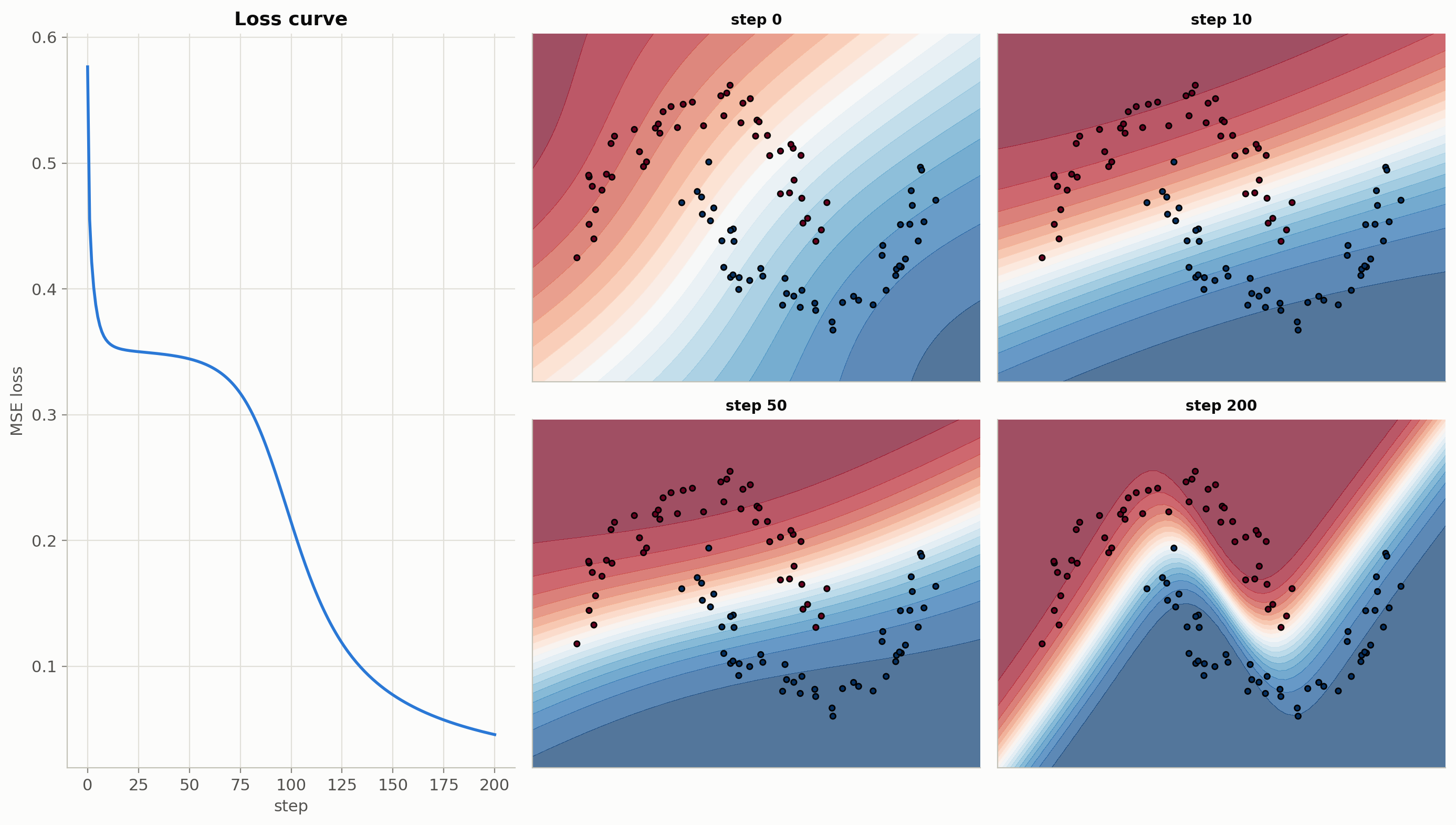
X, y = make_moons(n=100, noise=0.1, seed=0)targets =2.0* y -1.0# {0,1} -> {-1,+1} to pair with tanhdef batch_loss(model, X, targets): total =sum((model([*xi]).tanh() -float(ti)) **2for xi, ti inzip(X, targets))return total /len(X)model = MLP(2, [8, 1], seed=1)losses = []t0 = time.perf_counter()for step inrange(201): loss = batch_loss(model, X, targets) losses.append(loss.data) model.zero_grad() # chapter 01: grads accumulate unless reset loss.backward()for p in model.parameters(): p.data -=0.5* p.grad # lr = 0.5scalar_seconds = time.perf_counter() - t0print(f'loss: {losses[0]:.4f} -> {losses[-1]:.4f} 'f'({len(losses) -1} steps in {scalar_seconds:.1f}s on the scalar engine)')
loss: 0.5765 -> 0.0458 (200 steps in 7.4s on the scalar engine)
Plot: loss curve and the boundary taking shape
# Re-train with the same seed, capturing boundary grids at the snapshot steps.snap_steps = [0, 10, 50, 200]model = MLP(2, [8, 1], seed=1)gx, gy = np.meshgrid(np.linspace(X[:, 0].min() -0.4, X[:, 0].max() +0.4, 60), np.linspace(X[:, 1].min() -0.4, X[:, 1].max() +0.4, 60))grid = np.stack([gx.ravel(), gy.ravel()], axis=1)grids = {}for step inrange(201):if step in snap_steps: grids[step] = np.array([model([*g]).tanh().data for g in grid]).reshape(gx.shape) loss = batch_loss(model, X, targets) model.zero_grad(); loss.backward()for p in model.parameters(): p.data -=0.5* p.gradfig = plt.figure(figsize=(14, 8))ax = fig.add_subplot(2, 3, (1, 4))ax.plot(losses)ax.set_xlabel('step'); ax.set_ylabel('MSE loss'); ax.set_title('Loss curve')for i, step inenumerate(snap_steps): ax = fig.add_subplot(2, 3, [2, 3, 5, 6][i]) ax.contourf(gx, gy, grids[step], levels=20, cmap='RdBu', alpha=0.7) ax.scatter(X[:, 0], X[:, 1], c=y, cmap='RdBu', edgecolors='k', s=14) ax.set_title(f'step {step}', fontsize=10); ax.set_xticks([]); ax.set_yticks([])plt.tight_layout()plt.show()
3. The learning rate: the one knob you always tune
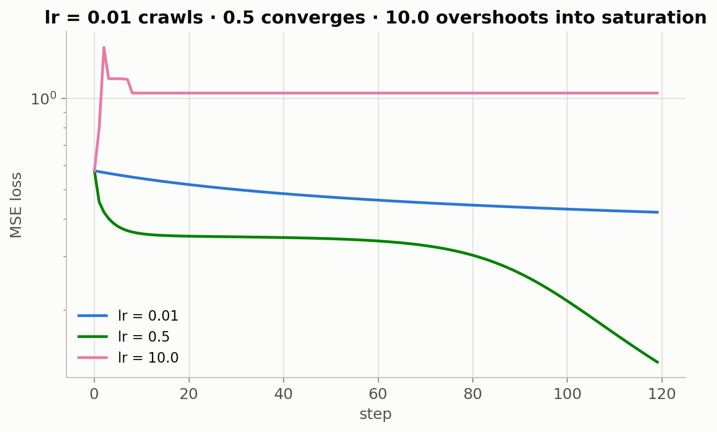
Same model, same data, three learning rates. Too small and nothing visibly happens in the budget; too large and each step overshoots the minimum it aims at — here the overshoot slams the tanh neurons into saturation and the loss settles worse than it started (with an unbounded loss it would explode outright). Every real run you’ll do (including milestone M5’s schedule sweep on your own model) is a negotiation with this plot:
Code
plt.figure(figsize=(8, 4.5))for lr in [0.01, 0.5, 10.0]: m = MLP(2, [8, 1], seed=1) curve = []for step inrange(120): loss = batch_loss(m, X, targets) curve.append(loss.data) m.zero_grad(); loss.backward()for p in m.parameters(): p.data -= lr * p.grad plt.plot(curve, label=f'lr = {lr}')plt.xlabel('step'); plt.ylabel('MSE loss'); plt.yscale('log')plt.legend(); plt.title('lr = 0.01 crawls · 0.5 converges · 10.0 overshoots into saturation')plt.show()
4. Minibatches: noisier steps, more of them
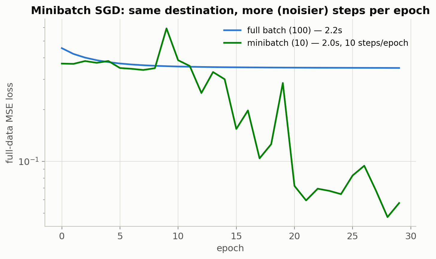
Full-batch descent computes the exact gradient — of a loss you only care about approximately. Stochastic gradient descent estimates it from a small random batch: each step is noisy, but you take 10 steps for the price of one, and the noise even helps escape flat regions. At LLM scale there is no choice: “full batch” would be the entire internet per step.
Code
def sgd_run(batch_size, epochs=30, lr=0.5, seed=1): m = MLP(2, [8, 1], seed=seed) r = np.random.default_rng(0) curve = []for _ inrange(epochs): order = r.permutation(len(X))for start inrange(0, len(X), batch_size): idx = order[start:start + batch_size] loss = batch_loss(m, X[idx], targets[idx]) m.zero_grad(); loss.backward()for p in m.parameters(): p.data -= lr * p.grad curve.append(batch_loss(m, X, targets).data) # full-data loss, once per epochreturn curvet0 = time.perf_counter(); full = sgd_run(batch_size=100); t_full = time.perf_counter() - t0t0 = time.perf_counter(); mini = sgd_run(batch_size=10); t_mini = time.perf_counter() - t0plt.figure(figsize=(8, 4.5))plt.plot(full, label=f'full batch (100) — {t_full:.1f}s')plt.plot(mini, label=f'minibatch (10) — {t_mini:.1f}s, 10 steps/epoch')plt.xlabel('epoch'); plt.ylabel('full-data MSE loss'); plt.yscale('log'); plt.legend()plt.title('Minibatch SGD: same destination, more (noisier) steps per epoch')plt.show()print(f'Same {len(full)} epochs: the minibatch run took 10x more steps 'f'({len(mini) *10} vs {len(full)}), each computed on 1/10th of the data.')
Same 30 epochs: the minibatch run took 10x more steps (300 vs 30), each computed on 1/10th of the data.
5. The PyTorch bridge
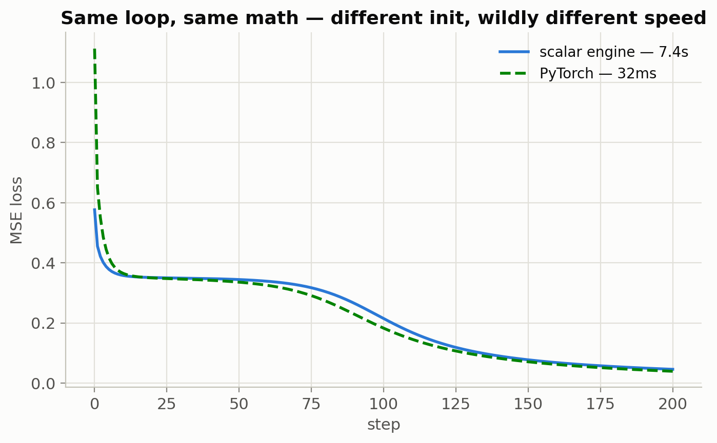
The same architecture and loop in PyTorch — nn.Sequential for the layers, optim.SGD wrapping the p.data -= lr * p.grad line, zero_grad() playing itself. Overlaid loss curves land on top of each other; the wall-clock does not, and that gap is the vectorization story from chapter 01:
PyTorch is ~233x faster here: same 201 steps, tensors instead of Python floats.
Key Takeaways
Training is five lines: forward, zero_grad, backward, step, repeat. Everything in training/trainer.py — and every trick in Phase 2 — is an upgrade to one of them.
zero_grad() is not optional: chapter 01’s accumulating gradients are a feature (gradient accumulation uses it deliberately) that becomes a bug if you forget the reset.
The learning rate has three regimes — crawl, converge, diverge — and the loss curve tells you which one you’re in at a glance.
Minibatch SGD trades gradient exactness for step count, and wins. Batch size is a systems knob as much as a statistics one — that tension returns in Gradient Accumulation.
Concrete numbers: 201 full-batch steps of a 33-parameter MLP on 100 points — a few seconds on the scalar engine, milliseconds in PyTorch (the printed ratio above, typically two to three orders of magnitude). Same math; tensors.
MSE on ±1 targets worked, but it was the wrong loss for classification. Why, and what the right one’s gradient looks like: Softmax & Cross-Entropy — with milestone M0.