A Virtual GPU: Watch a Tesla T4 Execute Your Kernel
The SIMT simulator answers what does my kernel do. This chapter answers why does it take this long — with a cycle-approximate model of a real card (the Tesla T4, the free GPU behind this notebook’s Colab badge) and a graphical view of the machine while it runs: 40 SMs lighting up, warps stalling on memory, a DRAM gauge saturating.
Design and honesty contract live in docs/VIRTUAL_GPU_SPEC.md. The short version: blocks become resident up to the occupancy limit, warp schedulers issue ready warps, DRAM ops park a warp for ~450 cycles and queue on one chip-wide bandwidth pipe priced by coalescing transactions, and barriers park warps until their block arrives. Latency hiding, the bandwidth wall, and block waves emerge from those rules — nothing below is scripted. The model predicts trends and ratios, never milliseconds; no caches, no ILP, no DRAM row effects.
Concepts covered
#
Concept
Section
1
The T4’s shape: SMs, warp slots, register file, bandwidth
Watch a virtual Tesla T4 execute kernels: occupancy, latency hiding, and the bandwidth wall, with a time axis.
🏗️ Chapter milestone: M11 — predict your model’s decode-step time on the virtual T4 — the exercise at the end of this chapter; see The Project.
Tip⏱️ Sessions S5.5–S5.6
Two sessions: S5.5 watches the virtual T4 execute; S5.6 is 🏗️ M11 — predict your decode step. Cards, prerequisites, and done-when tests: the Session Guide.
No GPU needed — the virtual T4 is pure Python + NumPy. (On Colab you can additionally run the real T4 counterparts from CUDA Basics for comparison.)
Setup
# Setup — works from a repo checkout (via ../src) or standalone on Colabimport syssys.path.insert(0, '../src')try:import ai_playground # noqa: F401exceptImportError:%pip install -q git+https://github.com/ggreg/ai_playground.git%config InlineBackend.figure_format ='retina'from ai_playground.plotting import apply_plot_styleapply_plot_style()
1. Meet the virtual T4
A GPU model is just numbers. Everything downstream — occupancy, timing, the animations — consumes this spec, so mimicking an A100 instead is one constant:
T4: 40 SMs x 64 lanes = 2560 CUDA cores, 8.1 FP32 TFLOPS
    32 warp slots/SM, 64K registers/SM, 64 KB shared/SM, 320 GB/s DRAM
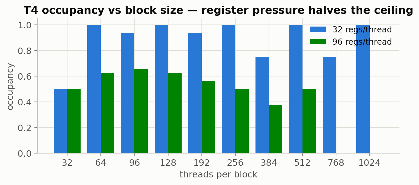
Occupancy — how many warps actually fit on an SM — is where launch configuration meets hardware. Four caps (warp slots, block slots, registers, shared memory) each limit resident blocks; the hardware takes the minimum. The calculator tells you which cap bound you:
256 threads, 32 regs         -> 100.0%, limited by warps
96 threads (indivisibility!)  -> 93.8%, limited by warps
256 threads, 96 regs         -> 50.0%, limited by registers
128 threads, 48 KB smem/blk  -> 12.5%, limited by shared
Show plotting code
import matplotlib.pyplot as pltfig, ax = plt.subplots(figsize=(8, 3))for regs, offset in [(32, -0.2), (96, 0.2)]: sweep = occupancy_sweep(T4, regs_per_thread=regs) xs = np.arange(len(sweep)) ax.bar(xs + offset, [o.occupancy for o in sweep], width=0.4, label=f'{regs} regs/thread')ax.set_xticks(np.arange(len(sweep)), [str(o.threads_per_block) for o in sweep])ax.set_xlabel('threads per block')ax.set_ylabel('occupancy')ax.set_title('T4 occupancy vs block size — register pressure halves the ceiling')ax.legend()plt.show()
Note 96-thread blocks: 93.75% with zero resource pressure — 3 warps per block simply doesn’t divide 32 slots. And at 96 registers/thread the ceiling halves everywhere: one extra register per thread can evict a whole block.
2. A first timed run
simulate() runs the kernel functionally (correctness + access log), then replays it through the machine model. Since Python kernels have no register allocator, you state what the real kernel would use (nvcc --ptxas-options=-v prints it; 32 is a typical default).
Read it like a profiler: ~63% of peak bandwidth achieved (real T4s land in the same range for plain copies), warp-cycles utterly dominated by stall_mem — a copy does no math — and occupancy capped at 50% because 32-thread blocks hit the 16-block slot limit first.
3. Latency hiding, watched happening
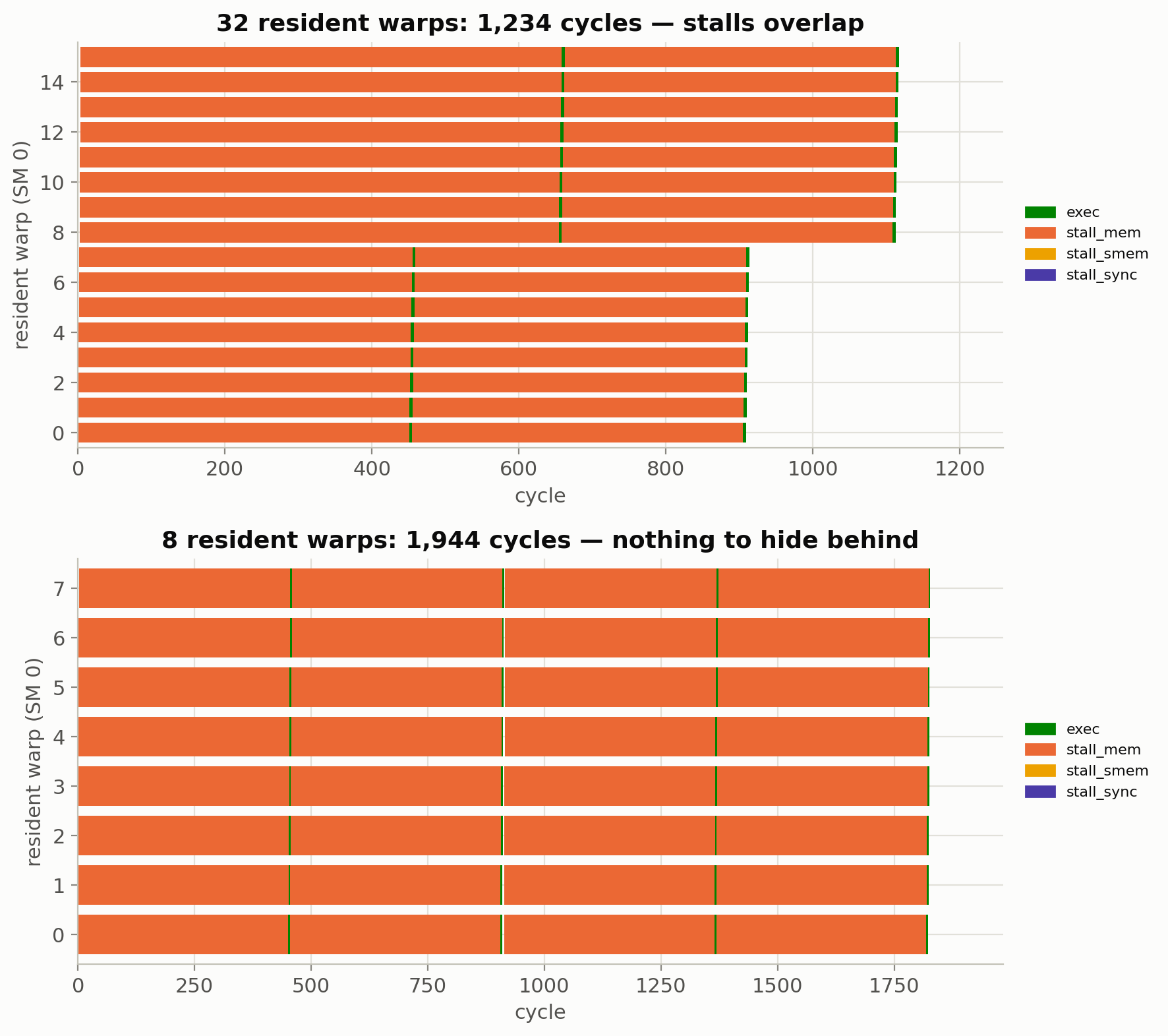
The waterfall shows one SM’s resident warps over time. Same kernel, same data — the only change is shared-memory pressure dropping residency from 4 blocks/SM to 1:
Nobody told the model that occupancy hides latency — it has warps, stalls, and schedulers, and the effect falls out. That is takeaway #5 of CUDA Basics, now as a picture.
4. The bandwidth wall, with a time axis
The SIMT chapter counted 32x transactions for strided access. Here’s what those transactions cost once enough data is in flight to saturate the pipe:
Note the strided run’s achieved bandwidth: the pipe is saturated — with garbage. 128 bytes cross the bus for every 4 useful ones. At small sizes this penalty mostly hides behind latency; at scale it is the wall. (Compare the real-hardware measurement in CUDA Basics §7.)
5. The die: block waves across 40 SMs
2,048 blocks, 640 resident at a time (16 block slots x 40 SMs) — the rest wave in as blocks retire. Green = executing, orange = stalled on DRAM, gray = empty slot; the right bar is the DRAM pipe gauge. Press play:
A copy kernel keeps the die orange — memory-bound by construction, exactly what §2’s summary said in numbers. A compute-heavy kernel would run green with an idle gauge.
6. Take a trace to a real profiler UI
Every trace exports to Chrome trace format — SMs as processes, warp slots as threads, one timestamp unit per cycle. Drop the file onto ui.perfetto.dev (or chrome://tracing) for pro-grade interactive scrubbing — the same viewer the repo’s PyTorch profiler wrapper targets:
Code
import tempfile, ospath = os.path.join(tempfile.gettempdir(), 't4_copy_trace.json')t_contig.to_chrome_json(path)print(f'wrote {path} ({os.path.getsize(path) /1e3:.0f} kB) — open it at https://ui.perfetto.dev')
wrote /var/folders/gm/lny259x17rjchmw201s4sfh80000gn/T/t4_copy_trace.json (600 kB) — open it at https://ui.perfetto.dev
7. Validate against the real card (Colab)
The spec’s standing checklist (docs/VIRTUAL_GPU_SPEC.md § Validation): hardware numbers via deviceQuery, then the trend experiments. These cells are skipped without CUDA — open this notebook on Colab (badge at the top, T4 runtime) and run them. Acceptance bar: rank order preserved, ratios within ~2× — a miss is shown, not hidden.
Code
import torchHAS_CUDA = torch.cuda.is_available()ifnot HAS_CUDA:print('No CUDA GPU here — open on Colab (T4 runtime) to run the validation.')else: p = torch.cuda.get_device_properties(0) checks = [ ('name contains T4', 'T4'in p.name, p.name), ('SM count', p.multi_processor_count == T4.n_sm, p.multi_processor_count), ('DRAM >= 15 GB', p.total_memory >15e9, f'{p.total_memory /1e9:.1f} GB'), ('compute capability 7.5', (p.major, p.minor) == (7, 5), f'{p.major}.{p.minor}'), ]for label, ok, got in checks:print(f'{"OK "if ok else"MISMATCH"}{label}: {got}')
No CUDA GPU here — open on Colab (T4 runtime) to run the validation.
Real-T4 trend experiments (numba) — run on Colab
if HAS_CUDA:import mathimport numpy as npfrom numba import cudadef gpu_ms(fn, *args, runs=20): fn(*args); cuda.synchronize() # warmup + JIT start, end = cuda.event(), cuda.event() start.record()for _ inrange(runs): fn(*args) end.record(); end.synchronize()return start.elapsed_time(end) / runs# --- trend 1: contiguous vs strided copy bandwidth ---@cuda.jitdef nb_copy(src, dst): i = cuda.grid(1)if i < dst.size: dst[i] = src[i]@cuda.jitdef nb_copy_strided(src, dst): i = cuda.grid(1)if i < dst.size: dst[i] = src[32* i] n =1<<24 d_src = cuda.to_device(np.zeros(32* n, np.float32)) d_dst = cuda.device_array(n, np.float32) blocks = math.ceil(n /256) ms_c = gpu_ms(lambda: nb_copy[blocks, 256](d_src, d_dst)) ms_s = gpu_ms(lambda: nb_copy_strided[blocks, 256](d_src, d_dst)) real_stride_ratio = ms_s / ms_c# --- simulator prediction for the same shape of experiment --- sim_c = simulate(copy, 1024, 32, (np.zeros(1024*32, np.float32), np.zeros(1024*32, np.float32))) sim_s = simulate(copy_strided, 1024, 32, (np.zeros(32*1024*32, np.float32), np.zeros(1024*32, np.float32))) sim_stride_ratio = sim_s.total_cycles / sim_c.total_cyclesprint(f'strided/contiguous slowdown: real T4 {real_stride_ratio:5.1f}x 'f'virtual T4 {sim_stride_ratio:5.1f}x 'f'{"PASS"if0.5< sim_stride_ratio / real_stride_ratio <2else"MISS (explain!)"}')# --- trend 2: achieved bandwidth on the contiguous copy --- real_gbps =2* n *4/ (ms_c *1e-3) /1e9print(f'contiguous copy bandwidth: real T4 {real_gbps:5.0f} GB/s 'f'virtual T4 {sim_c.achieved_bandwidth /1e9:5.0f} GB/s 'f'(theoretical peak {T4.dram_bandwidth /1e9:.0f})')else:print('skipped — no CUDA')
skipped — no CUDA
Record the numbers back into the spec doc when you run this — that closes the Phase-1/2 verification tasks. If a ratio misses the 2× bar, the interesting work is explaining which refusal (caches? DRAM row effects?) accounts for the gap.
🏗️ Project milestone M11 — predict your decode step
One decode step of your model at batch 8 moves roughly weight_bytes + 8 x kv_bytes(t) from DRAM. Simulate that traffic on the virtual T4 (a copy kernel sized to those bytes is a fair proxy for a memory-bound step), read predicted cycles and achieved GB/s from the trace summary, and convert to a predicted tokens/sec. Record it in metrics.json['m11_predicted'] — and if you’re on Colab, run the §7 validation cells and record the real bandwidth beside it.
Accept when: predicted decode tokens/sec is in metrics.json with the assumptions noted. Part of The Project: Serve Your Own LLM.
Session S5.6 — record m11_predicted = {'tokens_per_sec': …, 'assumptions': '…'}; verify: uv run pytest tests/milestones/test_m11_predicted.py.
Key Takeaways
Occupancy is a min over four caps — warp slots, block slots, registers (with 256/warp allocation granularity), shared memory — and knowing which cap binds tells you what to fix.
Latency hiding emerges from having enough warps. 32 resident warps absorb a ~450-cycle stall; 4 leave the SM idle — the model produces this, it doesn’t assert it.
Coalescing is a bandwidth-pipe tax. Strided access saturates DRAM with mostly-wasted bytes; the gauge shows a full pipe and a slow kernel simultaneously.
Blocks arrive in waves sized by occupancy x SM count; the die animation makes grid-size effects (tail waves, partial last wave) visible.
Cycle-approximate means ratios, not milliseconds. No caches, no ILP, no DRAM row effects — see the spec’s Refusals. Validate trends against the real T4 via the Colab badge; the spec’s validation table is the standing checklist.
What to read next
02_sgemm_optimization.ipynb — real CUDA on real hardware, where these effects become nanoseconds instead of colored pixels.
The engine: src/ai_playground/gpusim/timing.py (~200 lines) — small enough to read, and modifying it (add an L2? model dual-issue?) is a great exercise.