Chapter 00 ended with a network that had capacity but no knowledge. Knowledge enters through gradients: how much each of the (possibly billions of) parameters should move to reduce the loss. This chapter builds the machine that computes all of them at once:
Derivative = nudge — finite differences, the ground truth
The chain rule on a graph — gradients flow backward through composition
A Value class — ~60 lines that do what loss.backward() does
The PyTorch bridge — same expression, same gradients, assert allclose
Concepts covered
#
Concept
What to watch for
1
Finite differences
Slow but trustworthy — the oracle we check everything against
2
Computation graph
Every op records its inputs; the graph is the tape
3
Chain rule
Local derivative × downstream gradient, at every node
4
Gradient accumulation
grad +=, never = — the classic from-scratch bug
5
Topological order
Why a node’s _backward may only run after all its consumers
At milestone M4 you will type loss.backward() and train your own LLM (Training From Scratch). That one line is this chapter: reverse-mode differentiation over a recorded computation graph, vectorized. Owning the scalar version is what makes the later chapters mechanical rather than magical — mixed precision (chapter 2.2) is about where these gradients lose bits; gradient accumulation (2.3) is literally this chapter’s grad += across microbatches; the activation memory that pins your GPU budget is the graph this chapter records.
🏗️ Chapter milestone: none — but the engine built here is the one M0 (chapter 03) checks against PyTorch to six decimal places.
Tip⏱️ Session S0.2
One session: read and run everything, then verify one hand-derived gradient with Value. Cards, prerequisites, and done-when tests: the Session Guide.
Setup
# Setup — works from a repo checkout (via ../src) or standalone on Colabimport syssys.path.insert(0, '../src')try:import ai_playground # noqa: F401exceptImportError:%pip install -q git+https://github.com/ggreg/ai_playground.git%config InlineBackend.figure_format ='retina'from ai_playground.plotting import apply_plot_styleapply_plot_style()
Code
import mathimport matplotlib.pyplot as pltimport numpy as npimport torch
1. A derivative is a nudge
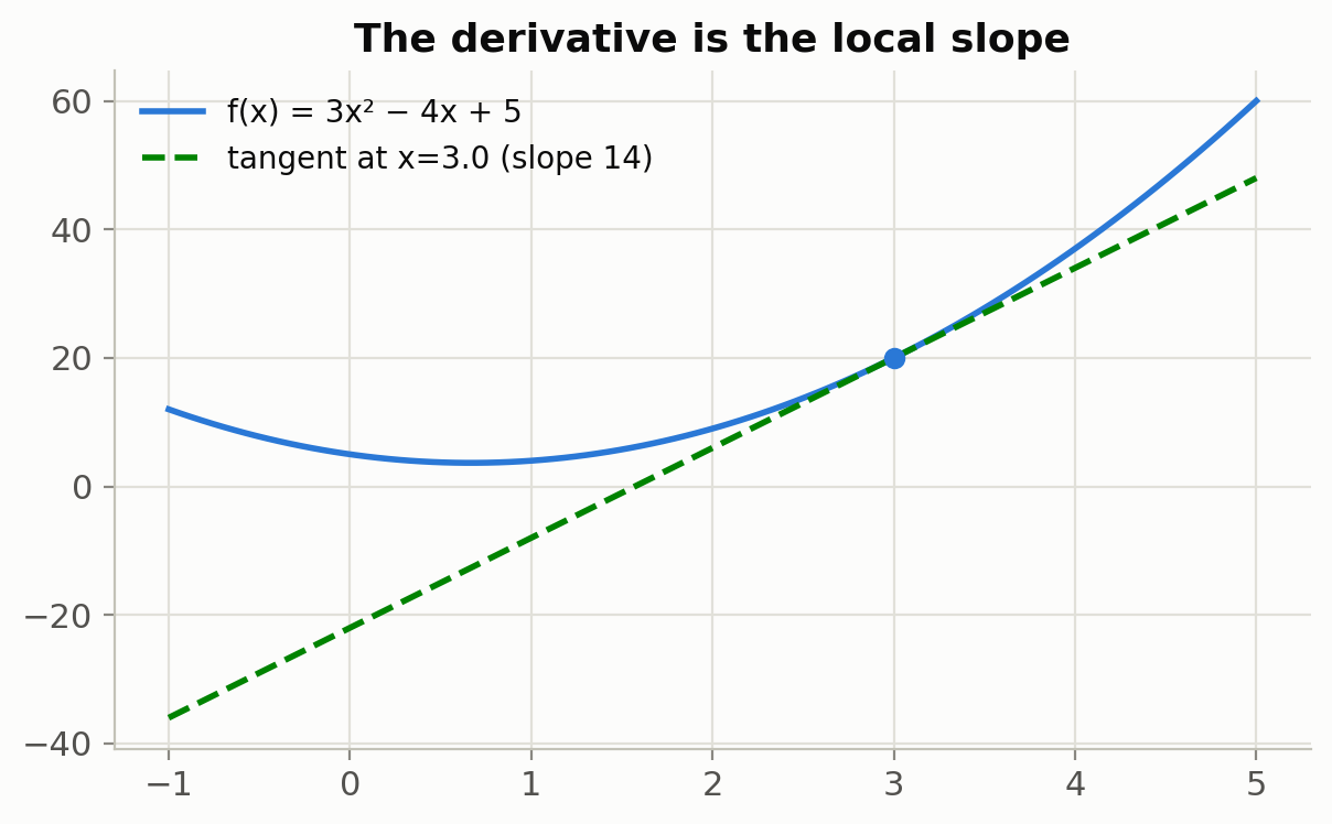
Forget symbols for a second: the derivative of f at x answers “if I nudge x a little, how much does f move?”. That definition is directly computable — nudge and measure. Finite differences are too slow to train with (one probe per parameter per step — 7 billion forward passes for one update of a 7B model), but they are simple enough to trust, which makes them our oracle for everything that follows.
Code
def f(x):return3* x**2-4* x +5x0, eps =3.0, 1e-6slope = (f(x0 + eps) - f(x0 - eps)) / (2* eps) # central differenceprint(f'numeric df/dx at {x0} = {slope:.6f}')print(f'analytic 6x - 4 at {x0} = {6* x0 -4:.6f}')xs = np.linspace(-1, 5, 100)plt.figure(figsize=(7, 4))plt.plot(xs, f(xs), label='f(x) = 3x² − 4x + 5')plt.plot(xs, f(x0) + slope * (xs - x0), '--', label=f'tangent at x={x0} (slope {slope:.0f})')plt.scatter([x0], [f(x0)], zorder=3)plt.legend()plt.title('The derivative is the local slope')plt.show()
numeric  df/dx at 3.0 = 14.000000
analytic 6x - 4 at 3.0 = 14.000000
2. The chain rule, on a graph
Real losses are compositions: L = g(f(x)). The chain rule says the sensitivities multiply along the path: dL/dx = dL/df · df/dx. Draw the computation as a graph and the rule becomes mechanical — each node multiplies the gradient flowing in from its output by its own local derivative, and passes the product to its inputs.
Notice what each variable needed to know: only its own local derivative and the gradient handed to it from downstream. Nothing global. That locality is what lets us automate the whole thing.
3. Build the engine: a Value that remembers
The plan, in three moves:
Each Value stores its number (data), the values that made it (_children), and a gradient slot (grad).
Each operation installs a _backward closure that does exactly what we did by hand: take out.grad, multiply by the local derivative, add into each input’s grad.
backward() visits nodes in reverse topological order — a node’s closure runs only after every consumer has deposited its share.
Why += and not =? If a value is used twice, each use contributes a path, and the total derivative is the sum of the paths. We’ll test exactly that case.
Code
class Value:"""A scalar that remembers how it was computed, so it can backpropagate."""def__init__(self, data, _children=(), _op=''):self.data =float(data)self.grad =0.0self._backward =lambda: Noneself._children = _childrenself._op = _opdef__add__(self, other): other = other ifisinstance(other, Value) else Value(other) out = Value(self.data + other.data, (self, other), '+')def _backward():self.grad += out.grad # local derivative of + is 1 other.grad += out.grad out._backward = _backwardreturn outdef__mul__(self, other): other = other ifisinstance(other, Value) else Value(other) out = Value(self.data * other.data, (self, other), '*')def _backward():self.grad += other.data * out.grad # d(ab)/da = b other.grad +=self.data * out.grad # d(ab)/db = a out._backward = _backwardreturn outdef__pow__(self, k): # k is a plain number out = Value(self.data**k, (self,), f'**{k}')def _backward():self.grad += k *self.data**(k -1) * out.grad out._backward = _backwardreturn outdef tanh(self): t = math.tanh(self.data) out = Value(t, (self,), 'tanh')def _backward():self.grad += (1- t * t) * out.grad out._backward = _backwardreturn outdef backward(self):# Topological sort: children before parents, so reversed() visits# each node only after ALL its consumers have pushed gradient into it. topo, visited = [], set()def build(v):ifid(v) notin visited: visited.add(id(v))for child in v._children: build(child) topo.append(v) build(self)self.grad =1.0# dL/dLfor v inreversed(topo): v._backward()def__repr__(self):returnf'Value(data={self.data:.4g}, grad={self.grad:.4g})'
Code
# The graph from section 2, now differentiated automatically:a, b, c = Value(2.0), Value(-3.0), Value(10.0)L = (a * b + c) **2L.backward()print(f'L = {L.data}')print(f'a: {a}') # expect grad -24print(f'b: {b}') # expect grad 16print(f'c: {c}') # expect grad 8
4. The bug everyone writes once: grad = vs grad +=
b = a + a uses a twice. Both paths contribute d b/d a = 1, so the true gradient is 2. An engine that assigns instead of accumulating silently reports 1 — wrong answers, no crash. The same diamond shape appears everywhere in real models: a weight reused across a batch, a residual stream feeding both a block and the skip connection.
Code
a = Value(3.0)(a + a).backward()print(f'd(a+a)/da = {a.grad} (both paths counted — with `=` this would be 1.0)')# Fresh node each backward: gradients accumulate across calls too, which is# exactly the behavior gradient accumulation (chapter 2.3) exploits on purpose.# It also means real training loops must zero_grad() between steps.
d(a+a)/da = 2.0 (both paths counted — with `=` this would be 1.0)
5. A full neuron, gradchecked
One tanh neuron — tanh(w1·x1 + w2·x2 + b) — backpropagated by the engine, every gradient verified against the nudge oracle from section 1:
Code
def neuron(w1, w2, b, x1=0.5, x2=-1.2):return (w1 * x1 + w2 * x2 + b).tanh()params = {'w1': Value(0.8), 'w2': Value(-0.3), 'b': Value(0.1)}out = neuron(**params)out.backward()eps =1e-6print(f'{"param":>5}{"engine":>12}{"finite diff":>12}')for name, p in params.items(): hi = {k: Value(v.data + (eps if k == name else0.0)) for k, v in params.items()} lo = {k: Value(v.data - (eps if k == name else0.0)) for k, v in params.items()} numeric = (neuron(**hi).data - neuron(**lo).data) / (2* eps)print(f'{name:>5}{p.grad:12.8f}{numeric:12.8f}')
PyTorch’s autograd is this algorithm with tensors instead of scalars: same graph recording, same reverse topological sweep, same accumulate-into-.grad. Identical expression, identical gradients:
Code
# Our enginea, b, c = Value(2.0), Value(-3.0), Value(10.0)L = ((a * b + c) **2).tanh()L.backward()# PyTorch, same expressionat = torch.tensor(2.0, dtype=torch.float64, requires_grad=True)bt = torch.tensor(-3.0, dtype=torch.float64, requires_grad=True)ct = torch.tensor(10.0, dtype=torch.float64, requires_grad=True)Lt = torch.tanh((at * bt + ct) **2)Lt.backward()for name, ours, theirs in [('a', a, at), ('b', b, bt), ('c', c, ct)]:assertabs(ours.grad - theirs.grad.item()) <1e-8print(f'd L/d {name}: Value {ours.grad:+.10f} torch {theirs.grad.item():+.10f}')print('\nSame algorithm. torch just runs it over tensors, on GPUs, in parallel.')
d L/d a:  Value -0.0000000000   torch -0.0000000000
d L/d b:  Value +0.0000000000   torch +0.0000000000
d L/d c:  Value +0.0000000000   torch +0.0000000000

Same algorithm. torch just runs it over tensors, on GPUs, in parallel.
The dictionary between the two, which you can now read in both directions:
our engine
PyTorch
notes
Value(2.0)
torch.tensor(2.0, requires_grad=True)
leaf node
_children, _op
grad_fn
the recorded graph
out._backward closure
a Function’s backward
local derivative rule
L.backward()
loss.backward()
reverse topological sweep
p.grad += ...
.grad accumulation
why optimizer.zero_grad() exists
p.grad = 0.0 loop
optimizer.zero_grad()
reset between steps
7. The engine, packaged
The polished version of this class — with relu, exp, log, division, and reversed operands — lives in src/ai_playground/fundamentals/autograd.py, and tests/test_fundamentals.py gradchecks every op against torch.autograd. From here on we import it:
Code
from ai_playground.fundamentals import Value as PackagedValuea = PackagedValue(2.0)L = (a *-3.0+10.0).tanh() /2.0+ (0.5* a).exp()L.backward()print(a)
Value(data=2, grad=1.35713)
Key Takeaways
Reverse mode is the whole trick: one backward sweep prices a nudge of every parameter at once — gradients for N parameters at ~the cost of one forward pass, which is why training a 7B-parameter model is possible at all (Rumelhart et al., 1986).
Every op is local: record inputs, define a local derivative, multiply by the incoming gradient. ~60 lines cover an MLP’s needs.
grad +=, never = — shared subexpressions sum their paths. The diamond test (b = a + a → a.grad == 2) catches the classic bug.
Topological order matters: a node backpropagates only after all its consumers have.
loss.backward() is this engine, vectorized — verified here by assert against torch.autograd, and in tests/test_fundamentals.py op by op.
A gradient is only useful if you step on it. Next: The Training Loop.