Mixture of Experts (MoE)

A standard transformer uses one FFN per layer. Every token goes through the same weights. Mixture of Experts replaces this single FFN with N expert FFNs and a router that picks which experts each token uses.

This lets you scale model parameters without scaling compute β€” each token only activates a small fraction of the total parameters.

Model Total params Active params per token Experts
LLaMA 3 70B 70B 70B (dense) 1 (standard FFN)
Mixtral 8x7B 47B 13B 8 experts, top-2 routing
DeepSeek-V2 236B 21B 160 experts, top-6 routing
GPT-4 (rumored) ~1.8T ~280B 16 experts, top-2 routing

This notebook covers: 1. Why MoE? β€” the scaling problem and how sparse experts solve it 2. The Router β€” how tokens choose their experts 3. Top-k expert selection β€” why we use 2 experts, not 1 or all 4. Load balancing β€” preventing expert collapse 5. Full MoE layer β€” from scratch, with visualizations 6. Comparison β€” dense vs MoE on our tiny model

References

TipπŸ“Ί Video companion

A Visual Guide to Mixture of Experts (Maarten Grootendorst) covers the routing, expert capacity, and load-balancing ideas this notebook implements β€” more in Videos.

Note🎯 Goal

Understand sparse expert FFNs: routing, load balancing, and the total-vs-active parameter distinction.

πŸ—οΈ Chapter milestone: M3 β€” decide dense vs MoE for your model, with the serving cost spelled out β€” the exercise at the end of this chapter; see The Project.

Tip⏱️ Session S1.4

One session, ending in πŸ—οΈ M3 β€” the dense-vs-MoE decision, with numbers. Cards, prerequisites, and done-when tests: the Session Guide.

Open in Colab

Setup
# Setup β€” works from a repo checkout (via ../src) or standalone on Colab
import sys
sys.path.insert(0, '../src')
try:
    import ai_playground  # noqa: F401
except ImportError:
    %pip install -q git+https://github.com/ggreg/ai_playground.git

%config InlineBackend.figure_format = 'retina'
from ai_playground.plotting import apply_plot_style
apply_plot_style()
Code
import sys
sys.path.insert(0, '../src')

import torch
import torch.nn as nn
import torch.nn.functional as F
import matplotlib.pyplot as plt
import matplotlib.patches as mpatches
import numpy as np
import math

from ai_playground.models.layers import SwiGLU

torch.manual_seed(42)
device = 'cpu'

1. Why MoE? The Scaling Problem

Making a model smarter means more parameters. But more parameters = more compute per token = slower inference.

MoE breaks this tradeoff: you can have 8Γ— more parameters while only using ~2Γ— more compute per token (by activating 2 out of 8 experts).

The key insight: not all knowledge is needed for every token. A math token needs different weights than a poetry token. Experts can specialize.

Show plotting code
# Visualize: Dense vs MoE architecture
fig, (ax1, ax2) = plt.subplots(1, 2, figsize=(16, 8))

# --- Left: Dense FFN ---
ax = ax1
ax.set_xlim(-1, 11)
ax.set_ylim(-1, 10)
ax.axis('off')
ax.set_title('Dense Transformer Block', fontsize=15, fontweight='bold')

def box(ax, x, y, w, h, label, color, sublabel=None, fontsize=11):
    rect = mpatches.FancyBboxPatch((x, y), w, h, boxstyle='round,pad=0.12',
                                    facecolor=color, edgecolor='#333', linewidth=1.5)
    ax.add_patch(rect)
    ax.text(x + w/2, y + h/2 + (0.15 if sublabel else 0), label,
            ha='center', va='center', fontsize=fontsize, fontweight='bold')
    if sublabel:
        ax.text(x + w/2, y + h/2 - 0.25, sublabel,
                ha='center', va='center', fontsize=8, color='#555')

def arrow(ax, x1, y1, x2, y2):
    ax.annotate('', xy=(x2, y2), xytext=(x1, y1),
                arrowprops=dict(arrowstyle='->', color='#333', lw=1.5))

# Input tokens
for i, tok in enumerate(['the', 'cat', 'sat']):
    box(ax, i*3.2 + 0.5, 8, 2.2, 0.7, tok, '#4ECDC4')

# Attention
arrow(ax, 5, 8, 5, 7.4)
box(ax, 1.5, 6.5, 7, 0.8, 'Multi-Head Attention', '#FF6B6B')

# Single FFN β€” all tokens go through same weights
arrow(ax, 5, 6.5, 5, 5.9)
box(ax, 1.5, 5, 7, 0.8, 'SwiGLU FFN (single)', '#95E1D3', 'ALL tokens use these same weights')

# Arrows from each token to FFN
for i in range(3):
    arrow(ax, i*3.2 + 1.6, 8, 5, 7.4)

ax.text(5, 4.0, f'Total params: N\nActive params: N\nEvery token uses 100% of FFN',
        ha='center', fontsize=11, color='#666',
        bbox=dict(boxstyle='round,pad=0.4', facecolor='#F1F5F9', edgecolor='#CBD5E1'))

# --- Right: MoE ---
ax = ax2
ax.set_xlim(-1, 11)
ax.set_ylim(-1, 10)
ax.axis('off')
ax.set_title('MoE Transformer Block', fontsize=15, fontweight='bold')

# Input tokens
for i, tok in enumerate(['the', 'cat', 'sat']):
    box(ax, i*3.2 + 0.5, 8, 2.2, 0.7, tok, '#4ECDC4')

# Attention
arrow(ax, 5, 8, 5, 7.4)
box(ax, 1.5, 6.5, 7, 0.8, 'Multi-Head Attention', '#FF6B6B')

# Router
arrow(ax, 5, 6.5, 5, 5.9)
box(ax, 2.5, 5.2, 5, 0.6, 'Router (learned)', '#FFE66D', 'picks top-k experts per token')

# Expert FFNs
expert_colors = ['#95E1D3', '#A8D8EA', '#B5EAD7', '#C7CEEA', '#E2F0CB', '#FFDAC1', '#FFB7B2', '#FF9AA2']
for i in range(4):
    x = i * 2.4 + 0.2
    box(ax, x, 3.0, 2.0, 0.7, f'Expert {i}', expert_colors[i], 'SwiGLU')

# Routing arrows β€” each token goes to 2 experts
routing = [(0, [0, 2]), (1, [1, 3]), (2, [0, 1])]  # token β†’ expert indices
route_colors = ['#4ECDC4', '#FF6B6B', '#C4B5FD']
for tok_i, (_, expert_ids) in enumerate(routing):
    for exp_i in expert_ids:
        x_start = tok_i * 3.2 + 1.6
        x_end = exp_i * 2.4 + 1.2
        ax.annotate('', xy=(x_end, 3.7), xytext=(x_start, 5.2),
                    arrowprops=dict(arrowstyle='->', color=route_colors[tok_i],
                                    lw=2, alpha=0.7))

ax.text(5, 1.5, f'Total params: 4N (4 experts)\nActive params: 2N (top-2 routing)\nEach token uses only 50% of FFN params',
        ha='center', fontsize=11, color='#666',
        bbox=dict(boxstyle='round,pad=0.4', facecolor='#F1F5F9', edgecolor='#CBD5E1'))

# Legend
for i, (tok, color) in enumerate(zip(['the', 'cat', 'sat'], route_colors)):
    ax.plot([], [], color=color, linewidth=2, label=f'"{tok}" β†’ experts')
ax.legend(loc='lower right', fontsize=10)

plt.tight_layout()
plt.show()

print('Left: Dense model β€” every token goes through the SAME FFN.')
print('Right: MoE model β€” router sends each token to its TOP-2 experts.')
print('4x parameters, but only 2x compute (since each token uses 2 of 4 experts).')

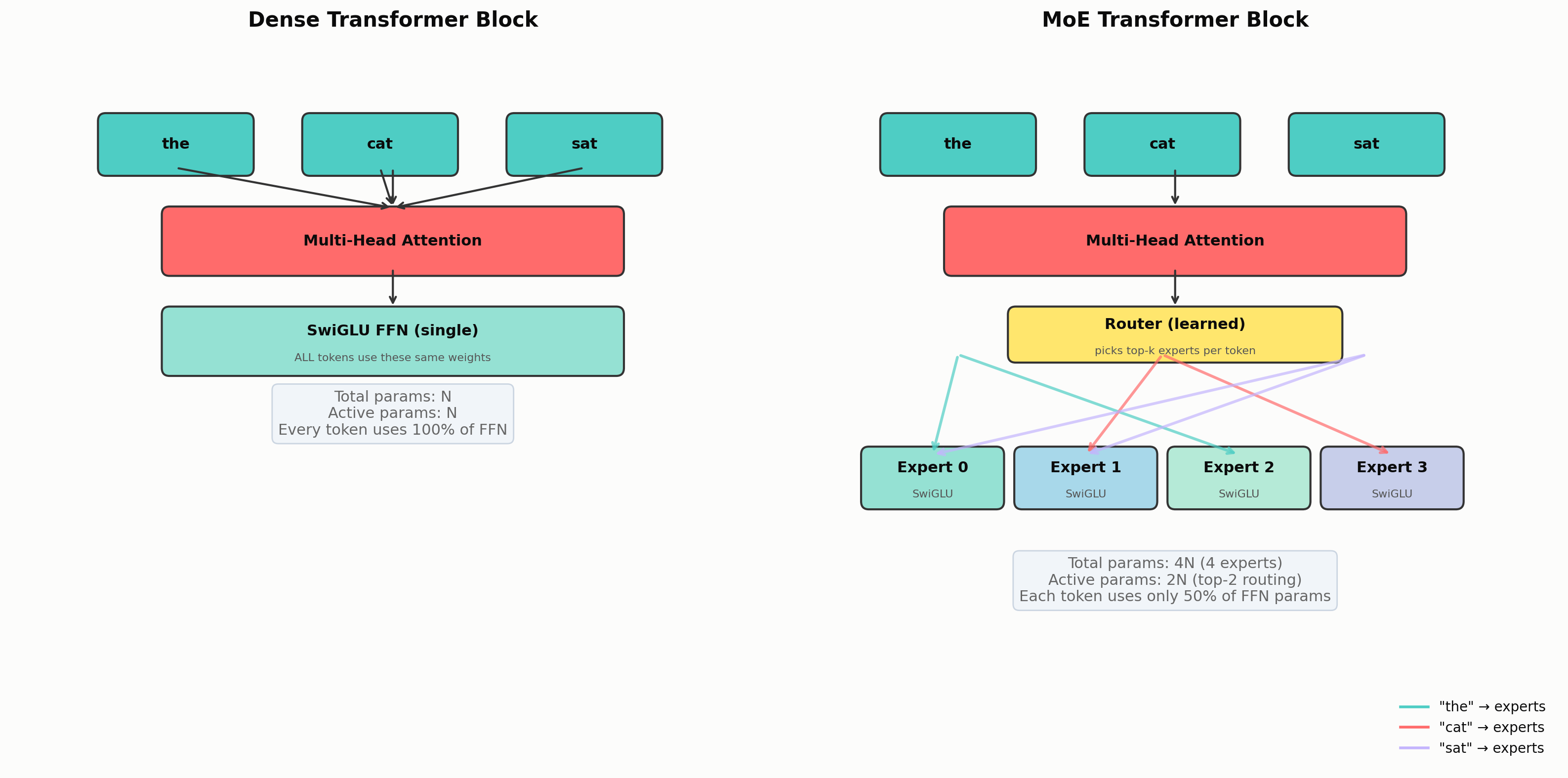
Left: Dense model β€” every token goes through the SAME FFN.
Right: MoE model β€” router sends each token to its TOP-2 experts.
4x parameters, but only 2x compute (since each token uses 2 of 4 experts).

2. The Router

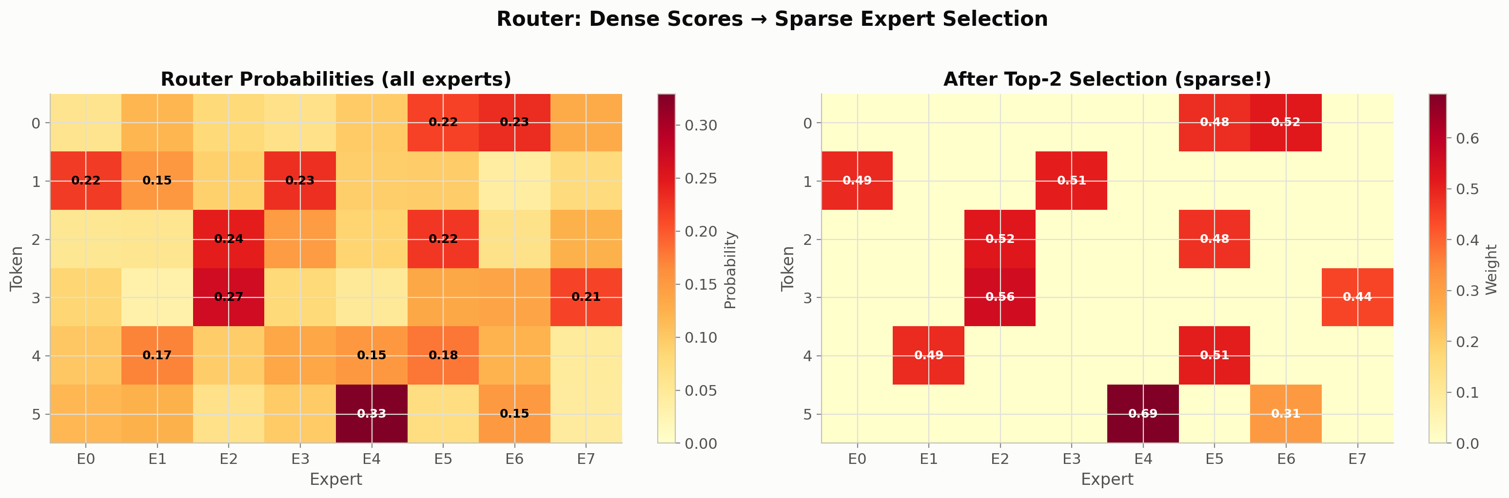
The router is a simple linear layer that scores each expert for each token:

router_scores = x @ W_router      # (batch, seq, n_experts)
router_probs  = softmax(scores)    # probability per expert
top_k_experts = topk(probs, k=2)   # pick the best 2

The router is learned β€” it trains alongside the model. Over time, it learns which expert patterns match which token patterns.

Switch Transformers showed that even k=1 (single expert per token) works well, but k=2 is more common in practice (Mixtral, DeepSeek) for better quality.

Code
# Build a router from scratch
class Router(nn.Module):
    """Token-to-expert routing via learned linear projection.
    
    Each token gets a score for each expert. We pick the top-k.
    
    References:
    - Switch Transformers: https://arxiv.org/abs/2101.03961
    - Mixtral: https://arxiv.org/abs/2401.04088
    """
    def __init__(self, dim: int, n_experts: int, top_k: int = 2):
        super().__init__()
        self.top_k = top_k
        self.gate = nn.Linear(dim, n_experts, bias=False)
    
    def forward(self, x: torch.Tensor):
        # x: (batch, seq, dim)
        scores = self.gate(x)                    # (batch, seq, n_experts)
        probs = F.softmax(scores, dim=-1)        # normalize to probabilities
        
        # Select top-k experts per token
        top_k_probs, top_k_indices = probs.topk(self.top_k, dim=-1)
        
        # Renormalize selected expert weights to sum to 1
        top_k_probs = top_k_probs / top_k_probs.sum(dim=-1, keepdim=True)
        
        return top_k_probs, top_k_indices, probs

# Demo
dim = 32
n_experts = 8
router = Router(dim, n_experts, top_k=2)

# Simulate 6 tokens
tokens = torch.randn(1, 6, dim)
top_k_probs, top_k_indices, all_probs = router(tokens)

print(f'Router: {dim}-dim input β†’ {n_experts} expert scores β†’ top-2 selection\n')
print(f'All expert probabilities (6 tokens Γ— 8 experts):')
for i in range(6):
    probs_str = ' '.join(f'{p:.2f}' for p in all_probs[0, i].tolist())
    print(f'  Token {i}: [{probs_str}]')

print(f'\nSelected experts (top-2 per token):')
for i in range(6):
    experts = top_k_indices[0, i].tolist()
    weights = top_k_probs[0, i].tolist()
    print(f'  Token {i}: expert {experts[0]} ({weights[0]:.0%}) + expert {experts[1]} ({weights[1]:.0%})')
Router: 32-dim input β†’ 8 expert scores β†’ top-2 selection

All expert probabilities (6 tokens Γ— 8 experts):
  Token 0: [0.06 0.12 0.08 0.06 0.10 0.22 0.23 0.13]
  Token 1: [0.22 0.15 0.09 0.23 0.09 0.10 0.04 0.08]
  Token 2: [0.05 0.06 0.24 0.15 0.09 0.22 0.06 0.12]
  Token 3: [0.09 0.03 0.27 0.08 0.05 0.13 0.14 0.21]
  Token 4: [0.10 0.17 0.09 0.14 0.15 0.18 0.12 0.05]
  Token 5: [0.12 0.12 0.07 0.10 0.33 0.07 0.15 0.04]

Selected experts (top-2 per token):
  Token 0: expert 6 (52%) + expert 5 (48%)
  Token 1: expert 3 (51%) + expert 0 (49%)
  Token 2: expert 2 (52%) + expert 5 (48%)
  Token 3: expert 2 (56%) + expert 7 (44%)
  Token 4: expert 5 (51%) + expert 1 (49%)
  Token 5: expert 4 (69%) + expert 6 (31%)
Show plotting code
# Visualize router probabilities as a heatmap
fig, (ax1, ax2) = plt.subplots(1, 2, figsize=(16, 5))

# Left: full probability distribution
im = ax1.imshow(all_probs[0].detach().numpy(), cmap='YlOrRd', aspect='auto', vmin=0)
ax1.set_xlabel('Expert', fontsize=12)
ax1.set_ylabel('Token', fontsize=12)
ax1.set_xticks(range(n_experts))
ax1.set_xticklabels([f'E{i}' for i in range(n_experts)])
ax1.set_title('Router Probabilities (all experts)', fontsize=14, fontweight='bold')
plt.colorbar(im, ax=ax1, label='Probability')

# Annotate values
for i in range(6):
    for j in range(n_experts):
        val = all_probs[0, i, j].item()
        if val > 0.15:
            ax1.text(j, i, f'{val:.2f}', ha='center', va='center', fontsize=9,
                    fontweight='bold', color='white' if val > 0.3 else 'black')

# Right: selected experts only (sparse)
selected = torch.zeros(6, n_experts)
for i in range(6):
    for k in range(2):
        exp_idx = top_k_indices[0, i, k].item()
        selected[i, exp_idx] = top_k_probs[0, i, k].item()

im2 = ax2.imshow(selected.numpy(), cmap='YlOrRd', aspect='auto', vmin=0)
ax2.set_xlabel('Expert', fontsize=12)
ax2.set_ylabel('Token', fontsize=12)
ax2.set_xticks(range(n_experts))
ax2.set_xticklabels([f'E{i}' for i in range(n_experts)])
ax2.set_title('After Top-2 Selection (sparse!)', fontsize=14, fontweight='bold')
plt.colorbar(im2, ax=ax2, label='Weight')

for i in range(6):
    for j in range(n_experts):
        val = selected[i, j].item()
        if val > 0:
            ax2.text(j, i, f'{val:.2f}', ha='center', va='center', fontsize=9,
                    fontweight='bold', color='white' if val > 0.3 else 'black')

plt.suptitle('Router: Dense Scores β†’ Sparse Expert Selection', fontsize=15, fontweight='bold', y=1.02)
plt.tight_layout()
plt.show()

print(f'Each token uses {2}/{n_experts} = {2/n_experts:.0%} of experts.')
print(f'This is the "sparsity" that makes MoE efficient.')

Each token uses 2/8 = 25% of experts.
This is the "sparsity" that makes MoE efficient.

3. Full MoE Layer

Let’s build a complete MoE layer that replaces the standard FFN. Each expert is a SwiGLU FFN (same as in our dense model), but there are N of them, and each token only uses top-k.

Code
class MoELayer(nn.Module):
    """Mixture of Experts layer β€” replaces the dense FFN.
    
    Each expert is an independent SwiGLU FFN. The router picks
    top-k experts per token. Output = weighted sum of selected experts.
    
    References:
    - Mixtral: https://arxiv.org/abs/2401.04088
    - Switch Transformers: https://arxiv.org/abs/2101.03961
    - Original MoE: https://arxiv.org/abs/1701.06538
    """
    def __init__(self, dim: int, hidden_dim: int, n_experts: int = 8, top_k: int = 2):
        super().__init__()
        self.n_experts = n_experts
        self.top_k = top_k
        self.router = Router(dim, n_experts, top_k)
        
        # N independent expert FFNs
        self.experts = nn.ModuleList([
            SwiGLU(dim, hidden_dim) for _ in range(n_experts)
        ])
    
    def forward(self, x: torch.Tensor):
        """Forward pass with sparse expert routing.
        
        For each token:
        1. Router picks top-k experts and their weights
        2. Run token through selected experts only
        3. Output = weighted sum of expert outputs
        """
        batch, seq_len, dim = x.shape
        
        # Route: which experts for each token?
        top_k_probs, top_k_indices, all_probs = self.router(x)
        # top_k_probs: (batch, seq, top_k)
        # top_k_indices: (batch, seq, top_k)
        
        # Process each token through its selected experts
        # (In production, this is done with scatter/gather for GPU efficiency.
        #  Here we loop for clarity.)
        output = torch.zeros_like(x)
        
        for b in range(batch):
            for t in range(seq_len):
                token = x[b, t].unsqueeze(0)  # (1, dim)
                
                for k in range(self.top_k):
                    expert_idx = top_k_indices[b, t, k].item()
                    weight = top_k_probs[b, t, k]
                    
                    # Run through this expert and weight by router score
                    expert_output = self.experts[expert_idx](token.unsqueeze(0))
                    output[b, t] += weight * expert_output.squeeze(0).squeeze(0)
        
        return output, all_probs

# Build and test
dim = 32
hidden_dim = 64
n_experts = 8
top_k = 2

moe = MoELayer(dim, hidden_dim, n_experts, top_k)
x = torch.randn(1, 6, dim)

with torch.no_grad():
    out, probs = moe(x)

# Count parameters
dense_params = sum(p.numel() for p in SwiGLU(dim, hidden_dim).parameters())
moe_params = sum(p.numel() for p in moe.parameters())

print(f'MoE Layer: {n_experts} experts, top-{top_k} routing')
print(f'  Input:  {list(x.shape)}')
print(f'  Output: {list(out.shape)}  (same shape β€” drop-in FFN replacement)\n')
print(f'Parameter comparison:')
print(f'  Dense FFN:     {dense_params:>8,} params (1 expert)')
print(f'  MoE layer:     {moe_params:>8,} params ({n_experts} experts + router)')
print(f'  Ratio:         {moe_params/dense_params:.1f}x more params')
print(f'  Active params: {dense_params * top_k:>8,} per token ({top_k} experts)')
print(f'  Efficiency:    {top_k}/{n_experts} = {top_k/n_experts:.0%} of params used per token')
MoE Layer: 8 experts, top-2 routing
  Input:  [1, 6, 32]
  Output: [1, 6, 32]  (same shape β€” drop-in FFN replacement)

Parameter comparison:
  Dense FFN:        6,144 params (1 expert)
  MoE layer:       49,408 params (8 experts + router)
  Ratio:         8.0x more params
  Active params:   12,288 per token (2 experts)
  Efficiency:    2/8 = 25% of params used per token

4. Load Balancing: The Expert Collapse Problem

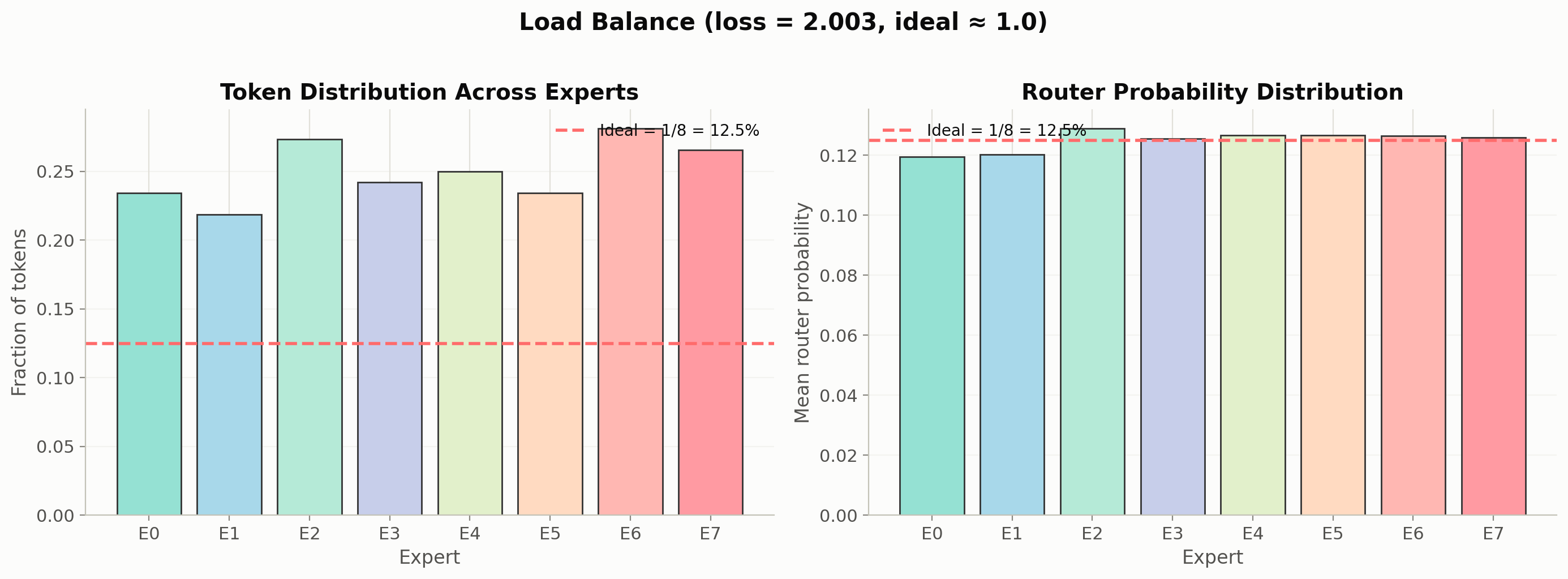
A naive router often learns to send all tokens to the same 1-2 experts, leaving the rest unused. This is called expert collapse β€” the model effectively shrinks to a dense model.

Auxiliary load balancing loss fixes this by penalizing uneven expert usage:

balance_loss = n_experts Γ— mean(fraction_per_expert) Γ— mean(prob_per_expert)

This encourages the router to spread tokens across experts. Switch Transformers introduced this as a lightweight add-on to the main cross-entropy loss (weighted by ~0.01).

Show plotting code
def compute_load_balance_loss(router_probs, top_k_indices, n_experts):
    """Auxiliary loss to prevent expert collapse.
    
    Encourages equal token distribution across experts.
    From Switch Transformers (https://arxiv.org/abs/2101.03961) Β§3.1.
    """
    # router_probs: (batch, seq, n_experts) β€” full probability distribution
    # top_k_indices: (batch, seq, top_k) β€” selected expert indices
    
    batch, seq_len = router_probs.shape[:2]
    total_tokens = batch * seq_len
    
    # Fraction of tokens assigned to each expert
    # (count how many tokens selected each expert)
    expert_mask = F.one_hot(top_k_indices, n_experts).sum(dim=2)  # (batch, seq, n_experts)
    fraction_per_expert = expert_mask.float().sum(dim=(0, 1)) / total_tokens
    
    # Average router probability per expert
    mean_prob_per_expert = router_probs.mean(dim=(0, 1))
    
    # Loss = n_experts * dot(fraction, mean_prob)
    # Minimized when both are uniform (1/n_experts each)
    balance_loss = n_experts * (fraction_per_expert * mean_prob_per_expert).sum()
    
    return balance_loss, fraction_per_expert, mean_prob_per_expert

# Visualize expert load distribution
torch.manual_seed(42)
moe_viz = MoELayer(dim, hidden_dim, n_experts=8, top_k=2)
x_viz = torch.randn(4, 32, dim)  # 4 batches Γ— 32 tokens = 128 tokens

with torch.no_grad():
    _, all_probs_viz = moe_viz(x_viz)
    _, top_k_idx_viz = all_probs_viz.topk(2, dim=-1)
    loss, frac, mean_p = compute_load_balance_loss(all_probs_viz, top_k_idx_viz, 8)

fig, (ax1, ax2) = plt.subplots(1, 2, figsize=(14, 5))

# Left: fraction of tokens per expert
colors_bar = [expert_colors[i] for i in range(8)]
ax1.bar(range(8), frac.numpy(), color=colors_bar, edgecolor='#333')
ax1.axhline(y=1/8, color='#FF6B6B', linestyle='--', linewidth=2, label=f'Ideal = 1/{8} = {1/8:.1%}')
ax1.set_xlabel('Expert', fontsize=12)
ax1.set_ylabel('Fraction of tokens', fontsize=12)
ax1.set_title('Token Distribution Across Experts', fontsize=14, fontweight='bold')
ax1.set_xticks(range(8))
ax1.set_xticklabels([f'E{i}' for i in range(8)])
ax1.legend(fontsize=10)
ax1.grid(True, alpha=0.3, axis='y')

# Right: average router probability per expert
ax2.bar(range(8), mean_p.numpy(), color=colors_bar, edgecolor='#333')
ax2.axhline(y=1/8, color='#FF6B6B', linestyle='--', linewidth=2, label=f'Ideal = 1/{8} = {1/8:.1%}')
ax2.set_xlabel('Expert', fontsize=12)
ax2.set_ylabel('Mean router probability', fontsize=12)
ax2.set_title('Router Probability Distribution', fontsize=14, fontweight='bold')
ax2.set_xticks(range(8))
ax2.set_xticklabels([f'E{i}' for i in range(8)])
ax2.legend(fontsize=10)
ax2.grid(True, alpha=0.3, axis='y')

plt.suptitle(f'Load Balance (loss = {loss.item():.3f}, ideal β‰ˆ 1.0)', fontsize=15, fontweight='bold', y=1.02)
plt.tight_layout()
plt.show()

print(f'Load balance loss: {loss.item():.3f}')
print(f'Ideal (uniform): 1.0')
print(f'Collapsed (all to 1 expert): {8:.1f}')
print(f'\nThe loss penalizes deviation from uniform β€” higher = more imbalanced.')

Load balance loss: 2.003
Ideal (uniform): 1.0
Collapsed (all to 1 expert): 8.0

The loss penalizes deviation from uniform β€” higher = more imbalanced.

5. Train Dense vs MoE: Side by Side

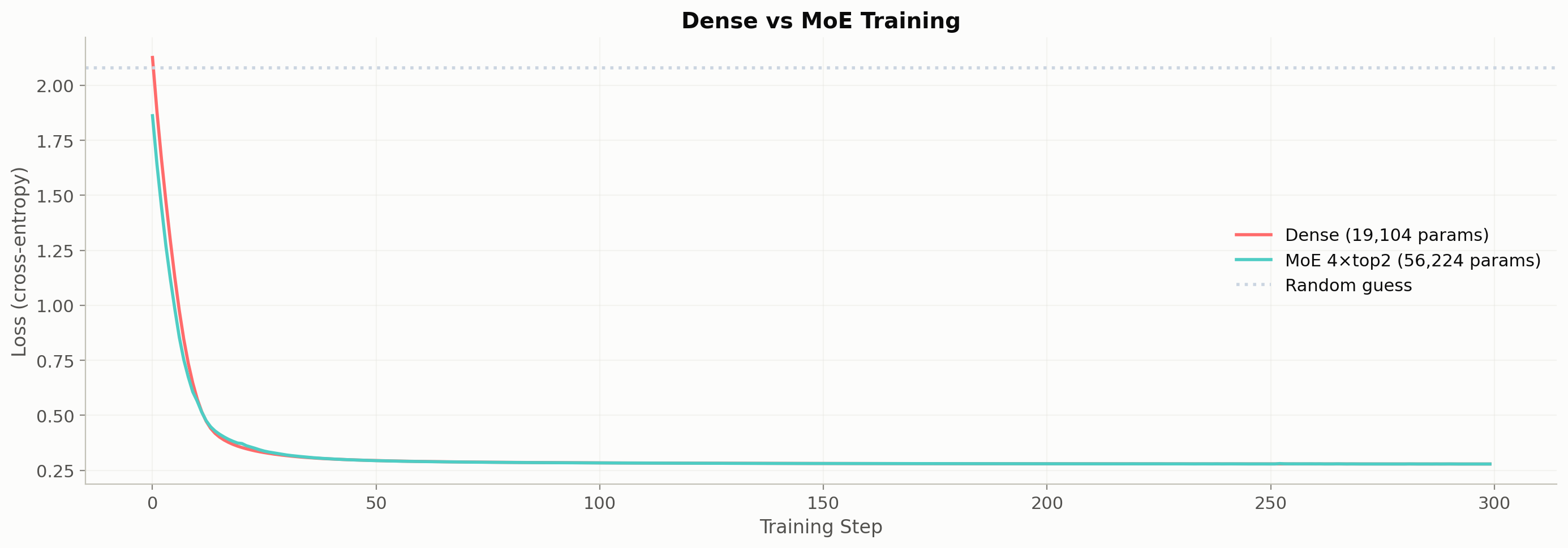
Let’s train two models on the same data: - Dense: standard SwiGLU FFN (like our regular transformer) - MoE: 4 expert FFNs with top-2 routing

Same total compute budget (the MoE model has more params but only activates 2 experts).

Code
from ai_playground.models.layers import RMSNorm
from ai_playground.models.attention import GroupedQueryAttention
from ai_playground.models import TransformerConfig
from ai_playground.models.layers import precompute_rope_frequencies

class TransformerBlockDense(nn.Module):
    """Standard transformer block with dense FFN."""
    def __init__(self, config):
        super().__init__()
        self.attention = GroupedQueryAttention(config)
        self.ffn = SwiGLU(config.dim, config.ffn_hidden_dim)
        self.norm1 = RMSNorm(config.dim)
        self.norm2 = RMSNorm(config.dim)
    
    def forward(self, x, freqs_cis, mask=None):
        x = x + self.attention(self.norm1(x), freqs_cis, mask)
        x = x + self.ffn(self.norm2(x))
        return x, None  # None = no aux loss

class TransformerBlockMoE(nn.Module):
    """Transformer block with MoE FFN."""
    def __init__(self, config, n_experts=4, top_k=2):
        super().__init__()
        self.attention = GroupedQueryAttention(config)
        self.moe = MoELayer(config.dim, config.ffn_hidden_dim, n_experts, top_k)
        self.norm1 = RMSNorm(config.dim)
        self.norm2 = RMSNorm(config.dim)
        self.n_experts = n_experts
    
    def forward(self, x, freqs_cis, mask=None):
        x = x + self.attention(self.norm1(x), freqs_cis, mask)
        moe_out, router_probs = self.moe(self.norm2(x))
        x = x + moe_out
        
        # Compute aux load balance loss
        _, top_k_idx = router_probs.topk(self.moe.top_k, dim=-1)
        aux_loss, _, _ = compute_load_balance_loss(router_probs, top_k_idx, self.n_experts)
        return x, aux_loss

class TinyTransformer(nn.Module):
    """Minimal transformer for dense vs MoE comparison."""
    def __init__(self, config, block_cls, **block_kwargs):
        super().__init__()
        self.config = config
        self.embed = nn.Embedding(config.vocab_size, config.dim)
        self.layers = nn.ModuleList([block_cls(config, **block_kwargs) for _ in range(config.n_layers)])
        self.norm = RMSNorm(config.dim)
        self.output = nn.Linear(config.dim, config.vocab_size, bias=False)
        self.register_buffer('freqs_cis',
            precompute_rope_frequencies(config.head_dim, config.max_seq_len))
    
    def forward(self, tokens):
        h = self.embed(tokens)
        freqs = self.freqs_cis[:tokens.shape[1]]
        total_aux = 0.0
        for layer in self.layers:
            h, aux = layer(h, freqs)
            if aux is not None:
                total_aux = total_aux + aux
        h = self.norm(h)
        return self.output(h), total_aux

# Config
config = TransformerConfig(
    vocab_size=8, dim=32, n_layers=2, n_heads=4,
    n_kv_heads=2, max_seq_len=16, ffn_dim_multiplier=2.0,
)

# Build both
torch.manual_seed(42)
model_dense = TinyTransformer(config, TransformerBlockDense)
torch.manual_seed(42)
model_moe = TinyTransformer(config, TransformerBlockMoE, n_experts=4, top_k=2)

params_dense = sum(p.numel() for p in model_dense.parameters())
params_moe = sum(p.numel() for p in model_moe.parameters())

print(f'Dense model: {params_dense:>8,} params')
print(f'MoE model:   {params_moe:>8,} params ({params_moe/params_dense:.1f}x more)')
print(f'MoE active:  ~{params_dense + (params_moe - params_dense) * 2 // 4:,} per token (2 of 4 experts)')
Dense model:   19,104 params
MoE model:     56,224 params (2.9x more)
MoE active:  ~37,664 per token (2 of 4 experts)
Show plotting code
# Training data
VOCAB = ['<pad>', 'the', 'cat', 'dog', 'sat', 'ran', 'on', 'mat']
tok2id = {t: i for i, t in enumerate(VOCAB)}
sentences = ['the cat sat on the mat', 'the dog ran on the mat',
             'the cat ran on the mat', 'the dog sat on the mat']
all_tok = [[tok2id[w] for w in s.split()] for s in sentences]
train_x = torch.tensor([t[:-1] for t in all_tok])
train_y = torch.tensor([t[1:] for t in all_tok])

def train_model(model, name, n_steps=300, aux_weight=0.01):
    optimizer = torch.optim.AdamW(model.parameters(), lr=3e-3)
    losses = []
    model.train()
    for step in range(n_steps):
        logits, aux_loss = model(train_x)
        ce_loss = F.cross_entropy(logits.view(-1, 8), train_y.view(-1))
        loss = ce_loss + aux_weight * aux_loss if isinstance(aux_loss, torch.Tensor) else ce_loss
        
        optimizer.zero_grad()
        loss.backward()
        optimizer.step()
        losses.append(ce_loss.item())
    
    print(f'{name:12s} | final loss: {losses[-1]:.4f}')
    return losses

losses_dense = train_model(model_dense, 'Dense')
losses_moe = train_model(model_moe, 'MoE (4Γ—top2)')

# Plot
fig, ax = plt.subplots(figsize=(14, 5))
ax.plot(losses_dense, label=f'Dense ({params_dense:,} params)', color='#FF6B6B', linewidth=2)
ax.plot(losses_moe, label=f'MoE 4Γ—top2 ({params_moe:,} params)', color='#4ECDC4', linewidth=2)
ax.axhline(y=np.log(8), color='#CBD5E1', linestyle=':', label='Random guess')
ax.set_xlabel('Training Step', fontsize=12)
ax.set_ylabel('Loss (cross-entropy)', fontsize=12)
ax.set_title('Dense vs MoE Training', fontsize=14, fontweight='bold')
ax.legend(fontsize=11)
ax.grid(True, alpha=0.3)
plt.tight_layout()
plt.show()

print(f'\nNote: On this tiny dataset, both converge quickly.')
print(f'The MoE advantage shows at scale β€” more params without proportional compute.')
Dense        | final loss: 0.2786
MoE (4Γ—top2) | final loss: 0.2786


Note: On this tiny dataset, both converge quickly.
The MoE advantage shows at scale β€” more params without proportional compute.

6. Expert Specialization

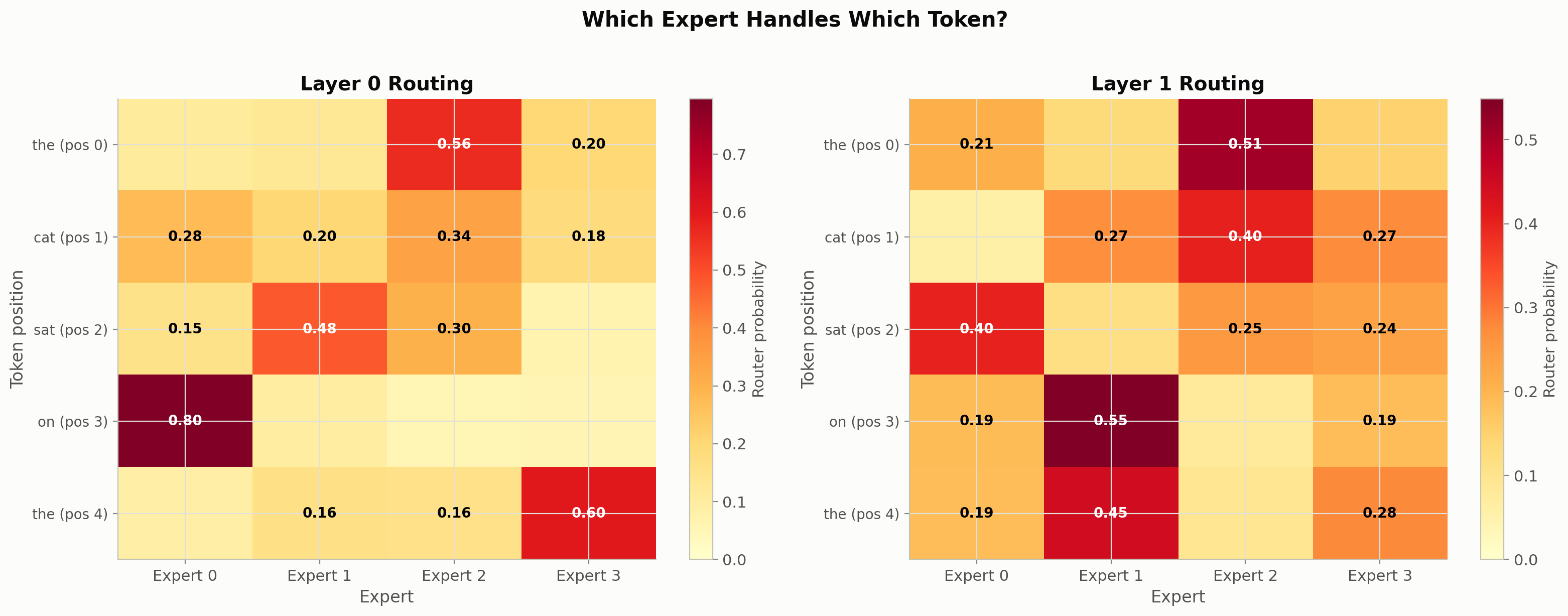
Do the experts actually learn different things? Let’s check which expert gets selected for which tokens after training.

Show plotting code
# Analyze routing after training
model_moe.eval()
with torch.no_grad():
    _, _ = model_moe(train_x)  # warm up
    
    # Collect routing decisions
    h = model_moe.embed(train_x)
    freqs = model_moe.freqs_cis[:train_x.shape[1]]
    
    all_routing = []
    for layer_idx, layer in enumerate(model_moe.layers):
        h_normed = layer.norm1(h)
        h = h + layer.attention(h_normed, freqs)
        h_normed2 = layer.norm2(h)
        _, router_probs = layer.moe(h_normed2)
        all_routing.append(router_probs)
        moe_out, _ = layer.moe(h_normed2)
        h = h + moe_out

id2tok = {i: t for t, i in tok2id.items()}

fig, axes = plt.subplots(1, 2, figsize=(16, 6))

for layer_idx, (ax, probs) in enumerate(zip(axes, all_routing)):
    # Average routing across all 4 sentences
    avg_probs = probs.mean(dim=0)  # (seq_len=5, n_experts=4)
    
    im = ax.imshow(avg_probs.numpy(), cmap='YlOrRd', aspect='auto', vmin=0)
    ax.set_xlabel('Expert', fontsize=12)
    ax.set_ylabel('Token position', fontsize=12)
    ax.set_xticks(range(4))
    ax.set_xticklabels([f'Expert {i}' for i in range(4)])
    ax.set_yticks(range(5))
    
    # Label with actual token names (from first sentence)
    token_labels = [id2tok[train_x[0, i].item()] for i in range(5)]
    ax.set_yticklabels([f'{tok} (pos {i})' for i, tok in enumerate(token_labels)], fontsize=10)
    ax.set_title(f'Layer {layer_idx} Routing', fontsize=14, fontweight='bold')
    plt.colorbar(im, ax=ax, label='Router probability')
    
    # Annotate
    for i in range(5):
        for j in range(4):
            val = avg_probs[i, j].item()
            if val > 0.15:
                ax.text(j, i, f'{val:.2f}', ha='center', va='center',
                        fontsize=10, fontweight='bold',
                        color='white' if val > 0.35 else 'black')

plt.suptitle('Which Expert Handles Which Token?', fontsize=15, fontweight='bold', y=1.02)
plt.tight_layout()
plt.show()

print('Different tokens may prefer different experts β€” this is specialization.')
print('The router learned this without any supervision β€” just from the training signal.')

Different tokens may prefer different experts β€” this is specialization.
The router learned this without any supervision β€” just from the training signal.

πŸ—οΈ Project milestone M3 β€” dense or MoE? Decide with numbers

Compute an MoE variant of your config (4 experts, top-1): total parameters vs active parameters per token. Then write down what serving it would cost you at M13: the mini-vLLM decode step batches the FFN across sequences β€” per-token routing breaks that batching, and expert weights multiply what streams from memory each step. Record the decision either way in checkpoints/myllm/DECISIONS.md with both parameter counts (dense is the recommended path; MoE is the ambitious one).

Accept when: DECISIONS.md exists with total/active numbers and one paragraph of reasoning. Part of The Project: Serve Your Own LLM.

Session S1.4 β€” write the entry under a ## M3 heading in DECISIONS.md; verify: uv run pytest tests/milestones/test_m03_decisions.py.

Key Takeaways

  1. MoE replaces the dense FFN with N expert FFNs + a learned router. Each token only uses top-k experts.
  2. More parameters, same compute: 8 experts with top-2 routing = 8Γ— params but only ~2Γ— compute per token.
  3. The router is a simple linear layer that learns to match tokens to experts via softmax scores.
  4. Load balancing prevents expert collapse β€” an auxiliary loss encourages uniform expert utilization.
  5. Experts specialize over training β€” different tokens route to different experts without supervision.
  6. MoE is how frontier models scale: Mixtral (8Γ—7B), DeepSeek-V2 (236B), and reportedly GPT-4 all use MoE.

When to use MoE vs Dense?

Dense MoE
Params vs compute Proportional Decoupled (more params, less compute)
Serving memory Lower Higher (all experts in memory)
Training stability Simpler Needs load balancing
Best for Smaller models, simpler setups Very large models (100B+)

References


πŸ”¨ From-scratch project: p1 β€” A tiny GPT from a blank file

This closes Phase 1: you’ve read every component of the architecture. The from-scratch project is to build a working decoder-only transformer in one file β€” no ai_playground.models, no nn.MultiheadAttention β€” well enough wired to pass a strict causality test and learn a deterministic copy task to near-zero loss.

Brief and rules: projects/p1_tiny_gpt/README.md

uv run pytest projects/p1_tiny_gpt/ -v