The learning rate (LR) is the most important hyperparameter in training. Too high → training diverges. Too low → training is painfully slow. The solution: change it during training.
This notebook covers: 1. Constant LR — the baseline (and why it’s not great) 2. Linear warmup — start small to avoid early instability 3. Cosine annealing — the standard for LLM training 4. Warmup + cosine — what we actually use (see trainer.py:93-102) 5. Impact on training — side-by-side comparison
Know why the learning rate changes during training and what warmup + cosine actually does to the loss.
🏗️ Chapter milestone: M5 — sweep schedules on your model and adopt the winner — the exercise at the end of this chapter; see The Project.
Tip⏱️ Session S2.4
One session, ending in 🏗️ M5 — sweep three schedules on your model, adopt the winner. Cards, prerequisites, and done-when tests: the Session Guide.
Setup
# Setup — works from a repo checkout (via ../src) or standalone on Colabimport syssys.path.insert(0, '../src')try:import ai_playground # noqa: F401exceptImportError:%pip install -q git+https://github.com/ggreg/ai_playground.git%config InlineBackend.figure_format ='retina'from ai_playground.plotting import apply_plot_styleapply_plot_style()
Code
import syssys.path.insert(0, '../src')import torchimport torch.nn as nnimport torch.nn.functional as Fimport matplotlib.pyplot as pltimport numpy as npimport mathfrom ai_playground.models import Transformer, TransformerConfigtorch.manual_seed(42)device ='cpu'
1. LR Schedule Zoo
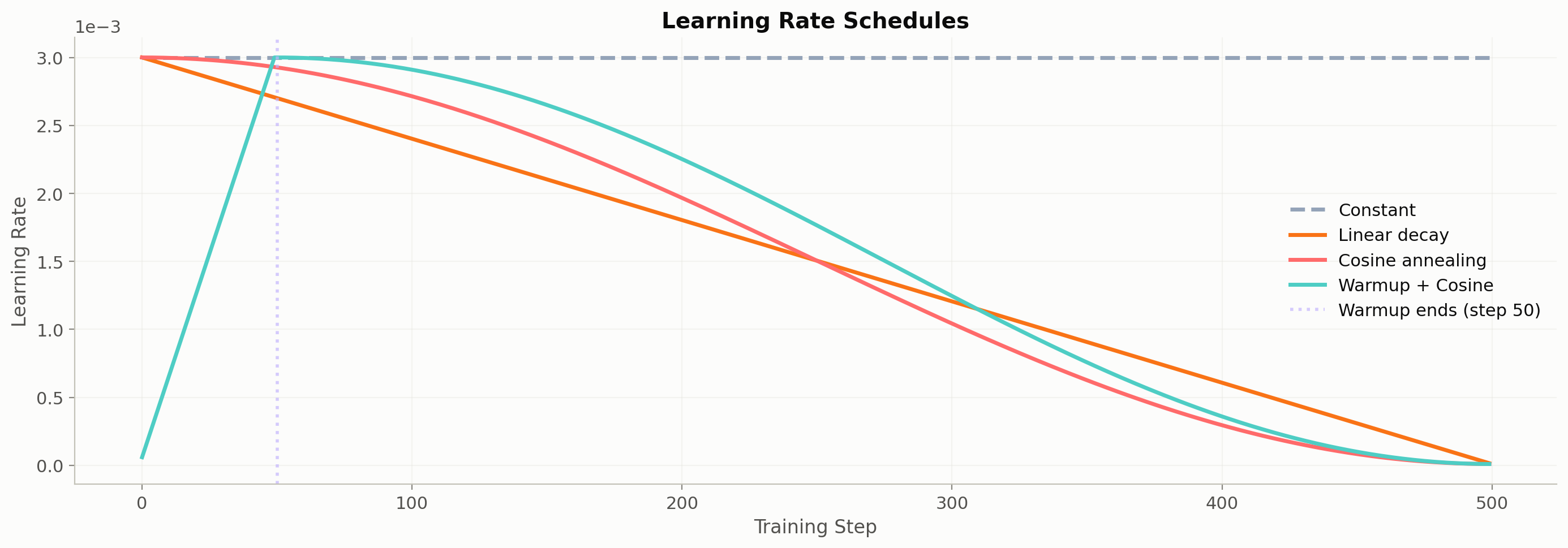
Let’s visualize the most common schedules. All of these start from a peak LR and decay over training — the question is how.
Show plotting code
max_steps =500warmup_steps =50peak_lr =3e-3min_lr =1e-5def schedule_constant(step):"""Constant LR — simple but suboptimal."""return peak_lrdef schedule_linear_decay(step):"""Linear decay from peak to min."""return peak_lr - (peak_lr - min_lr) * step / max_stepsdef schedule_cosine(step):"""Cosine annealing: smooth decay that slows down near the end. From SGDR (Loshchilov & Hutter, 2017): https://arxiv.org/abs/1608.03983 Widely adopted after GPT-2 and now standard for LLM training. """ progress = step / max_steps cosine =0.5* (1.0+ math.cos(math.pi * progress))return min_lr + (peak_lr - min_lr) * cosinedef schedule_warmup_cosine(step):"""Linear warmup + cosine decay — what we actually use. This is the schedule in trainer.py:93-102. Warmup described in "Attention Is All You Need" §5.3: https://arxiv.org/abs/1706.03762 """if step < warmup_steps:# Linear warmup: 0 → peak_lr over warmup_stepsreturn peak_lr * (step +1) / warmup_steps# Cosine decay: peak_lr → min_lr over remaining steps progress = (step - warmup_steps) / (max_steps - warmup_steps) cosine =0.5* (1.0+ math.cos(math.pi * progress))return min_lr + (peak_lr - min_lr) * cosine# Plot all schedulessteps =list(range(max_steps))schedules = [ ('Constant', schedule_constant, '#94A3B8', '--'), ('Linear decay', schedule_linear_decay, '#F97316', '-'), ('Cosine annealing', schedule_cosine, '#FF6B6B', '-'), ('Warmup + Cosine', schedule_warmup_cosine, '#4ECDC4', '-'),]fig, ax = plt.subplots(figsize=(14, 5))for name, fn, color, ls in schedules: lrs = [fn(s) for s in steps] ax.plot(steps, lrs, label=name, color=color, linewidth=2.5, linestyle=ls)ax.axvline(x=warmup_steps, color='#C4B5FD', linestyle=':', alpha=0.7, label=f'Warmup ends (step {warmup_steps})')ax.set_xlabel('Training Step', fontsize=12)ax.set_ylabel('Learning Rate', fontsize=12)ax.set_title('Learning Rate Schedules', fontsize=14, fontweight='bold')ax.legend(fontsize=11)ax.grid(True, alpha=0.3)ax.ticklabel_format(axis='y', style='scientific', scilimits=(-3, -3))plt.tight_layout()plt.show()print(f'Peak LR: {peak_lr}')print(f'Min LR: {min_lr}')print(f'Warmup steps: {warmup_steps}/{max_steps} ({warmup_steps/max_steps:.0%} of training)')
Peak LR: 0.003
Min LR: 1e-05
Warmup steps: 50/500 (10% of training)
2. Why Warmup?
At the start of training, the model’s weights are random. Gradients in this random landscape are noisy and can be very large. A high LR at this point pushes parameters far in unreliable directions → loss spikes or diverges.
Warmup starts with a tiny LR and ramps up over the first few hundred steps, giving the optimizer time to calibrate its momentum (the m and v in AdamW) before taking big steps.
Let’s demonstrate: train with and without warmup.
Code
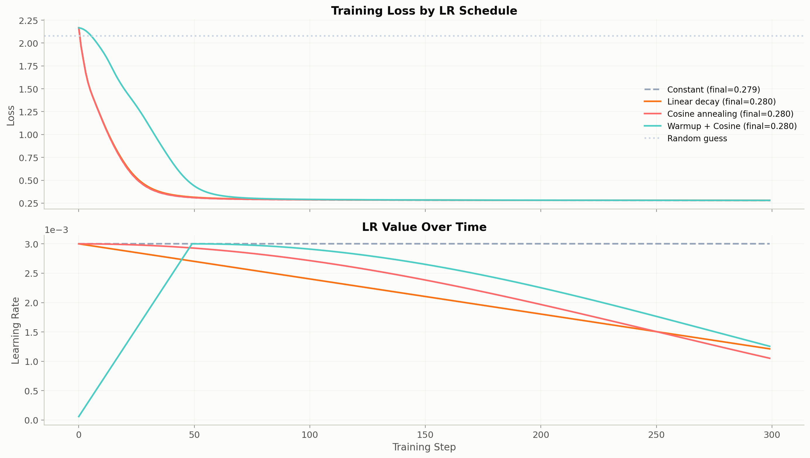
# Tiny vocabulary and data (same as overview notebook)VOCAB = ['<pad>', 'the', 'cat', 'dog', 'sat', 'ran', 'on', 'mat']tok2id = {t: i for i, t inenumerate(VOCAB)}id2tok = {i: t for t, i in tok2id.items()}sentences = ['the cat sat on the mat', 'the dog ran on the mat','the cat ran on the mat', 'the dog sat on the mat']def make_data(): all_tok = [[tok2id[w] for w in s.split()] for s in sentences] x = torch.tensor([t[:-1] for t in all_tok]) y = torch.tensor([t[1:] for t in all_tok])return x, ydef make_model(): cfg = TransformerConfig( vocab_size=len(VOCAB), dim=32, n_layers=2, n_heads=4, n_kv_heads=2, max_seq_len=16, ffn_dim_multiplier=2.0, )return Transformer(cfg).to(device)def train_with_schedule(schedule_fn, n_steps=300, seed=42):"""Train and return loss history.""" torch.manual_seed(seed) model = make_model() train_x, train_y = make_data() optimizer = torch.optim.AdamW(model.parameters(), lr=peak_lr) losses = [] lrs = [] model.train()for step inrange(n_steps): lr = schedule_fn(step)for pg in optimizer.param_groups: pg['lr'] = lr lrs.append(lr) logits = model(train_x) loss = F.cross_entropy(logits.view(-1, len(VOCAB)), train_y.view(-1)) optimizer.zero_grad() loss.backward() torch.nn.utils.clip_grad_norm_(model.parameters(), 1.0) optimizer.step() losses.append(loss.item())return losses, lrs# Compare schedulesresults = {}for name, fn, color, _ in schedules: results[name] = train_with_schedule(fn)print(f'{name:20s} | final loss: {results[name][0][-1]:.4f}')
Constant             | final loss: 0.2790
Linear decay         | final loss: 0.2801
Cosine annealing     | final loss: 0.2798
Warmup + Cosine      | final loss: 0.2802
Code
fig, (ax1, ax2) = plt.subplots(2, 1, figsize=(14, 8), sharex=True)for (name, fn, color, ls), (losses, lrs) inzip(schedules, results.values()): ax1.plot(losses, label=f'{name} (final={losses[-1]:.3f})', color=color, linewidth=2, linestyle=ls) ax2.plot(lrs, color=color, linewidth=2, linestyle=ls)ax1.axhline(y=np.log(len(VOCAB)), color='#CBD5E1', linestyle=':', label='Random guess')ax1.set_ylabel('Loss', fontsize=12)ax1.set_title('Training Loss by LR Schedule', fontsize=14, fontweight='bold')ax1.legend(fontsize=10)ax1.grid(True, alpha=0.3)ax2.set_xlabel('Training Step', fontsize=12)ax2.set_ylabel('Learning Rate', fontsize=12)ax2.set_title('LR Value Over Time', fontsize=14, fontweight='bold')ax2.grid(True, alpha=0.3)ax2.ticklabel_format(axis='y', style='scientific', scilimits=(-3, -3))plt.tight_layout()plt.show()print('\nObservations:')print('- Warmup + cosine typically gives the lowest final loss')print('- Constant LR can work but often overshoots near convergence')print('- Cosine without warmup may be unstable in early steps for larger models')
Observations:
- Warmup + cosine typically gives the lowest final loss
- Constant LR can work but often overshoots near convergence
- Cosine without warmup may be unstable in early steps for larger models
3. The Cosine Schedule in Detail
Why cosine specifically? Two reasons:
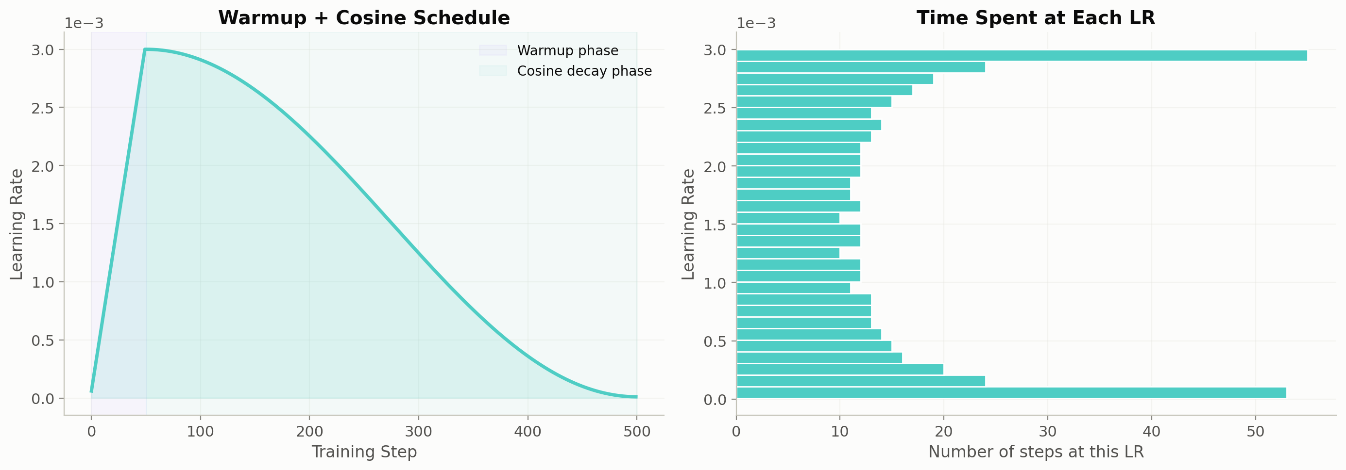
Spends more time at moderate LRs — the cosine curve is flat near the top and bottom, so the model trains longest at medium learning rates where it makes steady progress.
Smooth landing — gradual decay to near-zero avoids the loss spike you’d get from a sudden LR drop (step schedule) or the wasted compute from a too-fast linear decay.
# Visualize where the cosine schedule "spends its time"steps_arr = np.arange(max_steps)lrs_cosine = np.array([schedule_warmup_cosine(s) for s in steps_arr])fig, (ax1, ax2) = plt.subplots(1, 2, figsize=(14, 5))# Left: schedule with time-spent shadingax1.plot(steps_arr, lrs_cosine, color='#4ECDC4', linewidth=2.5)ax1.fill_between(steps_arr, 0, lrs_cosine, alpha=0.15, color='#4ECDC4')# Shade warmup regionax1.axvspan(0, warmup_steps, alpha=0.1, color='#C4B5FD', label='Warmup phase')ax1.axvspan(warmup_steps, max_steps, alpha=0.05, color='#4ECDC4', label='Cosine decay phase')ax1.set_xlabel('Training Step', fontsize=12)ax1.set_ylabel('Learning Rate', fontsize=12)ax1.set_title('Warmup + Cosine Schedule', fontsize=14, fontweight='bold')ax1.legend(fontsize=10)ax1.grid(True, alpha=0.3)ax1.ticklabel_format(axis='y', style='scientific', scilimits=(-3, -3))# Right: histogram of LR values (how many steps at each LR)ax2.hist(lrs_cosine, bins=30, color='#4ECDC4', edgecolor='white', orientation='horizontal')ax2.set_xlabel('Number of steps at this LR', fontsize=12)ax2.set_ylabel('Learning Rate', fontsize=12)ax2.set_title('Time Spent at Each LR', fontsize=14, fontweight='bold')ax2.grid(True, alpha=0.3)ax2.ticklabel_format(axis='y', style='scientific', scilimits=(-3, -3))plt.tight_layout()plt.show()print('The histogram shows cosine spends MORE time at moderate LRs')print('and less time at the extremes — a good property for stable training.')
The histogram shows cosine spends MORE time at moderate LRs
and less time at the extremes — a good property for stable training.
4. How to Choose the Peak LR
The peak LR depends on model size and batch size. Common values for LLM training:
Model size
Typical peak LR
~100M params
3e-4 to 6e-4
~1B params
1.5e-4 to 3e-4
~7B params
1e-4 to 1.5e-4
~70B params
1e-5 to 3e-5
Larger models need smaller LRs because they have more parameters interacting — a step that’s fine for a small model can destabilize a large one.
The Chinchilla paper (Hoffmann et al., 2022) also derived scaling laws for optimal LR based on model/data size.
Code
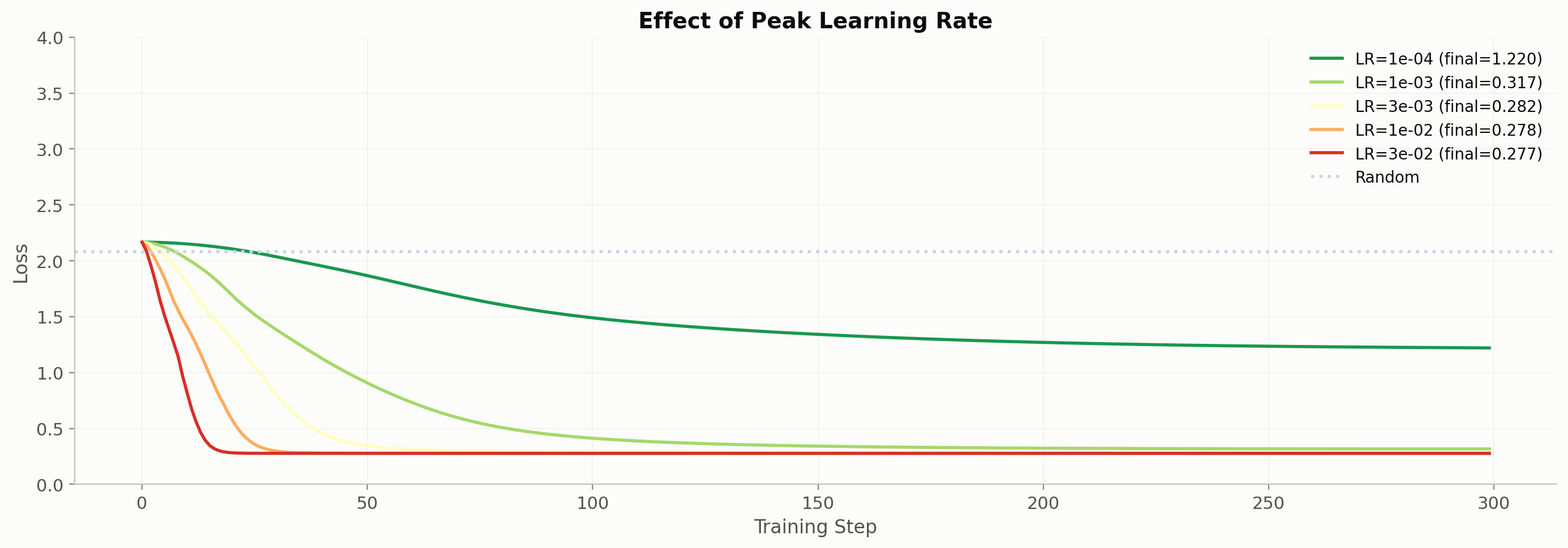
# Experiment: train with different peak LRspeak_lrs_to_try = [1e-4, 1e-3, 3e-3, 1e-2, 3e-2]colors_lr = plt.cm.RdYlGn_r(np.linspace(0.1, 0.9, len(peak_lrs_to_try)))fig, ax = plt.subplots(figsize=(14, 5))for peak, color inzip(peak_lrs_to_try, colors_lr):def make_schedule(peak=peak):def fn(step): ws =30if step < ws:return peak * (step +1) / ws progress = (step - ws) / (300- ws) cosine =0.5* (1+ math.cos(math.pi * progress))return min_lr + (peak - min_lr) * cosinereturn fn losses, _ = train_with_schedule(make_schedule(), n_steps=300) ax.plot(losses, label=f'LR={peak:.0e} (final={losses[-1]:.3f})', color=color, linewidth=2)ax.axhline(y=np.log(len(VOCAB)), color='#CBD5E1', linestyle=':', label='Random')ax.set_xlabel('Training Step', fontsize=12)ax.set_ylabel('Loss', fontsize=12)ax.set_title('Effect of Peak Learning Rate', fontsize=14, fontweight='bold')ax.legend(fontsize=10, loc='upper right')ax.grid(True, alpha=0.3)ax.set_ylim(0, max(4, np.log(len(VOCAB)) +0.5))plt.tight_layout()plt.show()print('Too low → learns slowly. Too high → unstable or diverges.')print('The sweet spot is typically found by trying 3-5 values on a small run.')
Too low → learns slowly. Too high → unstable or diverges.
The sweet spot is typically found by trying 3-5 values on a small run.
🏗️ Project milestone M5 — choose your schedule
Sweep three schedules on your model — constant, cosine, warmup+cosine — 200 steps each from the same seed and init. Append the results to the project log:
Accept when: metrics.json holds all three final losses and the chosen schedule is also recorded in config.json. Part of The Project: Serve Your Own LLM.
Session S2.4 — record the adopted schedule as "schedule": "<chosen>" in config.json; verify: uv run pytest tests/milestones/test_m05_schedule.py.
Key Takeaways
Warmup + cosine annealing is the standard LR schedule for LLM training.
Warmup (first 1-10% of steps) prevents early instability by letting the optimizer’s momentum estimates stabilize.
Cosine decay spends more time at moderate LRs and lands smoothly at the minimum.
Peak LR scales inversely with model size — larger models need smaller steps.
The schedule is implemented in trainer.py:93-102 using the exact formula shown above.