This notebook walks through the complete training pipeline, building each piece from first principles before using the library versions:
Data loading — how training data is prepared and batched
The training loop — forward pass, loss, backward pass, optimizer step
Cross-entropy loss — why this is the right loss for next-token prediction
Gradient descent — how parameters get updated
We use the same tiny 8-token vocabulary from 01_transformer_internals/00_transformer_overview.ipynb so you can focus on the training mechanics, not the data.
Run the full training loop — data, loss, backward, optimizer step — and read a loss curve like an instrument.
🏗️ Chapter milestone: M4 — the first real training run of your model — the exercise at the end of this chapter; see The Project.
Tip⏱️ Sessions S2.1–S2.3
Three sessions: S2.1 reads and runs the chapter; S2.2 is 🏗️ M4a (your config’s smoke run); S2.3 is 🏗️ M4b (the 300-step curve, diagnosed). Cards, prerequisites, and done-when tests: the Session Guide.
Setup
# Setup — works from a repo checkout (via ../src) or standalone on Colabimport syssys.path.insert(0, '../src')try:import ai_playground # noqa: F401exceptImportError:%pip install -q git+https://github.com/ggreg/ai_playground.git%config InlineBackend.figure_format ='retina'from ai_playground.plotting import apply_plot_styleapply_plot_style()
Code
import syssys.path.insert(0, '../src')import torchimport torch.nn as nnimport torch.nn.functional as Fimport matplotlib.pyplot as pltimport matplotlib.gridspec as gridspecimport numpy as npimport mathimport timefrom ai_playground.models import Transformer, TransformerConfigtorch.manual_seed(42)device ='cpu'
1. Preparing Training Data
Language model training uses next-token prediction: given a sequence of tokens, predict the next one at every position simultaneously.
Input:   the  cat  sat  on  the
Target:  cat  sat  on   the mat
The target is just the input shifted by one position. This is how the model learns language — by trying to predict what comes next, billions of times.
See src/ai_playground/training/data.py for the TextDataset implementation.
Code
# Our tiny vocabularyVOCAB = ['<pad>', 'the', 'cat', 'dog', 'sat', 'ran', 'on', 'mat']tok2id = {t: i for i, t inenumerate(VOCAB)}id2tok = {i: t for t, i in tok2id.items()}vocab_size =len(VOCAB)def tokenize(s):return [tok2id[w] for w in s.split()]# Training sentencessentences = ['the cat sat on the mat','the dog ran on the mat','the cat ran on the mat','the dog sat on the mat',]# Build input/target pairs: input[t] predicts target[t] = input[t+1]all_tokens = [tokenize(s) for s in sentences]train_x = torch.tensor([t[:-1] for t in all_tokens]) # (4, 5)train_y = torch.tensor([t[1:] for t in all_tokens]) # (4, 5)print('Next-token prediction setup:')print(f' Batch size: {train_x.shape[0]}, Sequence length: {train_x.shape[1]}\n')for i inrange(len(sentences)): inp = [id2tok[j.item()] for j in train_x[i]] tgt = [id2tok[j.item()] for j in train_y[i]]for pos inrange(len(inp)):print(f' Given [{" ".join(inp[:pos+1])}] → predict "{tgt[pos]}"')print()
Next-token prediction setup:
  Batch size: 4, Sequence length: 5

  Given [the] → predict "cat"
  Given [the cat] → predict "sat"
  Given [the cat sat] → predict "on"
  Given [the cat sat on] → predict "the"
  Given [the cat sat on the] → predict "mat"

  Given [the] → predict "dog"
  Given [the dog] → predict "ran"
  Given [the dog ran] → predict "on"
  Given [the dog ran on] → predict "the"
  Given [the dog ran on the] → predict "mat"

  Given [the] → predict "cat"
  Given [the cat] → predict "ran"
  Given [the cat ran] → predict "on"
  Given [the cat ran on] → predict "the"
  Given [the cat ran on the] → predict "mat"

  Given [the] → predict "dog"
  Given [the dog] → predict "sat"
  Given [the dog sat] → predict "on"
  Given [the dog sat on] → predict "the"
  Given [the dog sat on the] → predict "mat"
2. The Training Loop — Step by Step
Every training step has four phases:
Forward pass: input → model → logits (predictions)
Loss: compare predictions to targets → single number measuring “how wrong”
Backward pass: compute gradients (how to adjust each parameter to reduce loss)
Optimizer step: update parameters using gradients
Let’s do this manually first, then use the Trainer class.
Code
# Build a tiny modelconfig = TransformerConfig( vocab_size=vocab_size, dim=32, n_layers=2, n_heads=4, n_kv_heads=2, max_seq_len=16, ffn_dim_multiplier=2.0,)model = Transformer(config).to(device)print(f'Model: {sum(p.numel() for p in model.parameters()):,} parameters\n')# ============ Step 1: Forward pass ============# Feed tokens through the model to get logits (one score per vocab token)logits = model(train_x) # (batch=4, seq=5, vocab=8)print(f'1. FORWARD PASS')print(f' Input shape: {train_x.shape} (batch, seq_len)')print(f' Output shape: {logits.shape} (batch, seq_len, vocab_size)')print(f' Each position produces {vocab_size} scores — one per vocab token\n')# Show raw logits for first sentence, first positionprint(f' Raw logits at position 0 (after "the"):')for j, v inenumerate(VOCAB):print(f' {v:>5s}: {logits[0, 0, j].item():+.3f}')print()# ============ Step 2: Loss ============# Cross-entropy loss: measures how surprised the model is by the correct answer# Reshape for PyTorch: (batch*seq, vocab) vs (batch*seq,)loss = F.cross_entropy(logits.view(-1, vocab_size), train_y.view(-1))print(f'2. LOSS')print(f' Cross-entropy loss: {loss.item():.4f}')print(f' Random guessing would give: ln({vocab_size}) = {math.log(vocab_size):.4f}')print(f' Perfect predictions would give: ~0.0')print(f' Current model is {"worse than"if loss.item() > math.log(vocab_size) else"better than"} random\n')# ============ Step 3: Backward pass ============# Compute gradients: for each parameter, how does changing it affect the loss?loss.backward()# Show gradient statistics for one layerfirst_param =list(model.parameters())[0]print(f'3. BACKWARD PASS')print(f' Gradients computed for all {sum(1for p in model.parameters()):} parameter tensors')print(f' Example: embedding layer gradient shape = {first_param.grad.shape}')print(f' Gradient magnitude (L2 norm): {first_param.grad.norm().item():.6f}')print(f' This tells us the direction to nudge each parameter\n')# ============ Step 4: Optimizer step ============# AdamW updates parameters using gradients + momentumoptimizer = torch.optim.AdamW(model.parameters(), lr=1e-3)# Snapshot a weight beforew_before = model.tok_embeddings.weight[1].clone() # "the" embeddingoptimizer.step()optimizer.zero_grad()w_after = model.tok_embeddings.weight[1] # after updatew_delta = (w_after - w_before).norm().item()print(f'4. OPTIMIZER STEP (AdamW)')print(f' Embedding for "the" moved by {w_delta:.6f} (L2 distance)')print(f' Every parameter shifted slightly to reduce the loss')print(f' Repeat this 1000s of times → model learns the patterns')
Model: 19,104 parameters

1. FORWARD PASS
   Input shape:  torch.Size([4, 5])  (batch, seq_len)
   Output shape: torch.Size([4, 5, 8])  (batch, seq_len, vocab_size)
   Each position produces 8 scores — one per vocab token

   Raw logits at position 0 (after "the"):
     <pad>: +0.016
       the: +0.160
       cat: -0.095
       dog: -0.080
       sat: +0.094
       ran: +0.181
        on: -0.125
       mat: -0.015

2. LOSS
   Cross-entropy loss: 2.1666
   Random guessing would give: ln(8) = 2.0794
   Perfect predictions would give: ~0.0
   Current model is worse than random

3. BACKWARD PASS
   Gradients computed for all 21 parameter tensors
   Example: embedding layer gradient shape = torch.Size([8, 32])
   Gradient magnitude (L2 norm): 1.754817
   This tells us the direction to nudge each parameter

4. OPTIMIZER STEP (AdamW)
   Embedding for "the" moved by 0.005657 (L2 distance)
   Every parameter shifted slightly to reduce the loss
   Repeat this 1000s of times → model learns the patterns
3. Cross-Entropy Loss Explained
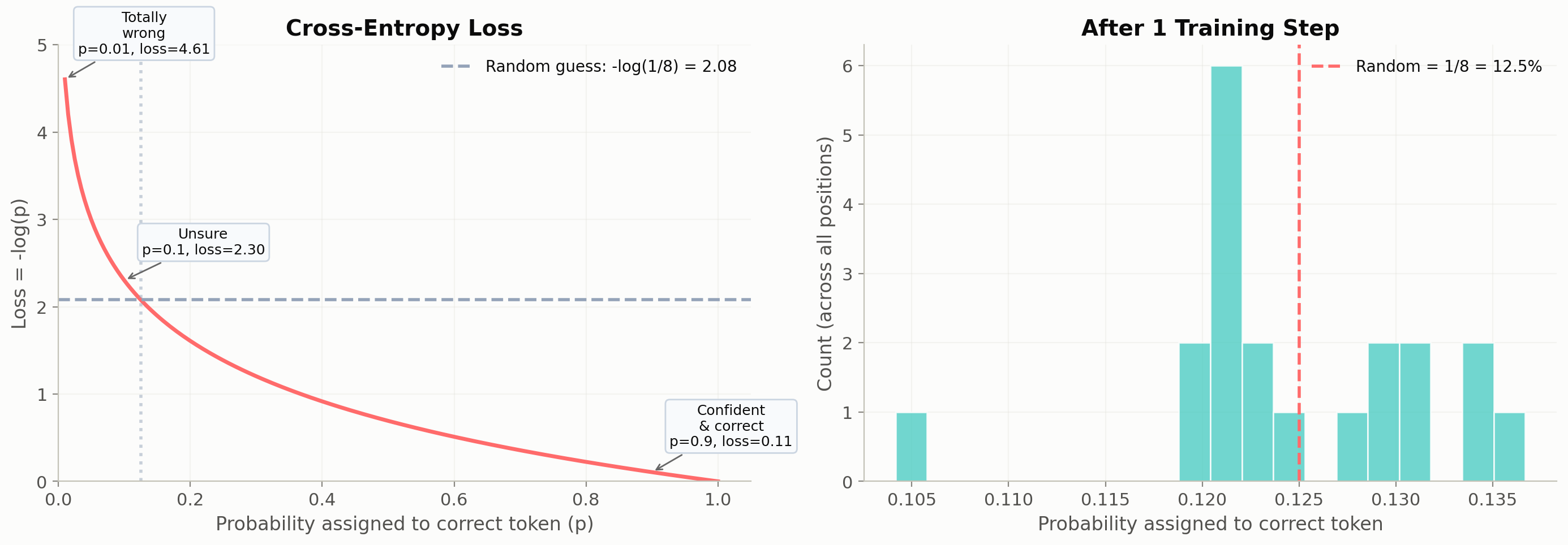
Cross-entropy measures how surprised the model is by the correct answer.
If the model assigns probability p to the correct token, the loss for that position is -log(p): - Model is 90% confident on the right answer → loss = -log(0.9) = 0.105 (low, good!) - Model is 10% confident → loss = -log(0.1) = 2.303 (high, bad!) - Random guessing (1/8 = 12.5% per token) → loss = -log(1/8) = 2.079
The total loss is averaged across all positions and all sentences in the batch.
Show plotting code
# Visualize cross-entropy loss functionfig, (ax1, ax2) = plt.subplots(1, 2, figsize=(14, 5))# Left: -log(p) curvep = np.linspace(0.01, 1.0, 200)ax1.plot(p, -np.log(p), color='#FF6B6B', linewidth=2.5)ax1.axhline(y=-np.log(1/vocab_size), color='#94A3B8', linestyle='--', label=f'Random guess: -log(1/{vocab_size}) = {-np.log(1/vocab_size):.2f}')ax1.axvline(x=1/vocab_size, color='#94A3B8', linestyle=':', alpha=0.5)ax1.set_xlabel('Probability assigned to correct token (p)', fontsize=12)ax1.set_ylabel('Loss = -log(p)', fontsize=12)ax1.set_title('Cross-Entropy Loss', fontsize=14, fontweight='bold')ax1.legend(fontsize=10)ax1.grid(True, alpha=0.3)ax1.set_xlim(0, 1.05)ax1.set_ylim(0, 5)# Annotate key pointsfor prob, label in [(0.9, 'Confident\n& correct'), (0.1, 'Unsure'), (0.01, 'Totally\nwrong')]: loss_val =-np.log(prob) ax1.annotate(f'{label}\np={prob}, loss={loss_val:.2f}', xy=(prob, loss_val), fontsize=9, ha='center', xytext=(prob +0.12, loss_val +0.3), arrowprops=dict(arrowstyle='->', color='#666'), bbox=dict(boxstyle='round,pad=0.3', facecolor='#F8FAFC', edgecolor='#CBD5E1'))# Right: compare loss before and after some trainingwith torch.no_grad(): logits_now = model(train_x) probs_now = F.softmax(logits_now, dim=-1)# Gather probabilities assigned to the correct target tokenscorrect_probs = probs_now.gather(2, train_y.unsqueeze(-1)).squeeze(-1) # (4, 5)all_probs = correct_probs.flatten().numpy()ax2.hist(all_probs, bins=20, color='#4ECDC4', edgecolor='white', alpha=0.8)ax2.axvline(x=1/vocab_size, color='#FF6B6B', linestyle='--', linewidth=2, label=f'Random = 1/{vocab_size} = {1/vocab_size:.1%}')ax2.set_xlabel('Probability assigned to correct token', fontsize=12)ax2.set_ylabel('Count (across all positions)', fontsize=12)ax2.set_title('After 1 Training Step', fontsize=14, fontweight='bold')ax2.legend(fontsize=10)ax2.grid(True, alpha=0.3)plt.tight_layout()plt.show()print(f'Average probability on correct token: {all_probs.mean():.1%}')print(f'Random would be: {1/vocab_size:.1%}')
Average probability on correct token: 12.5%
Random would be: 12.5%
4. Gradient Descent Visualized
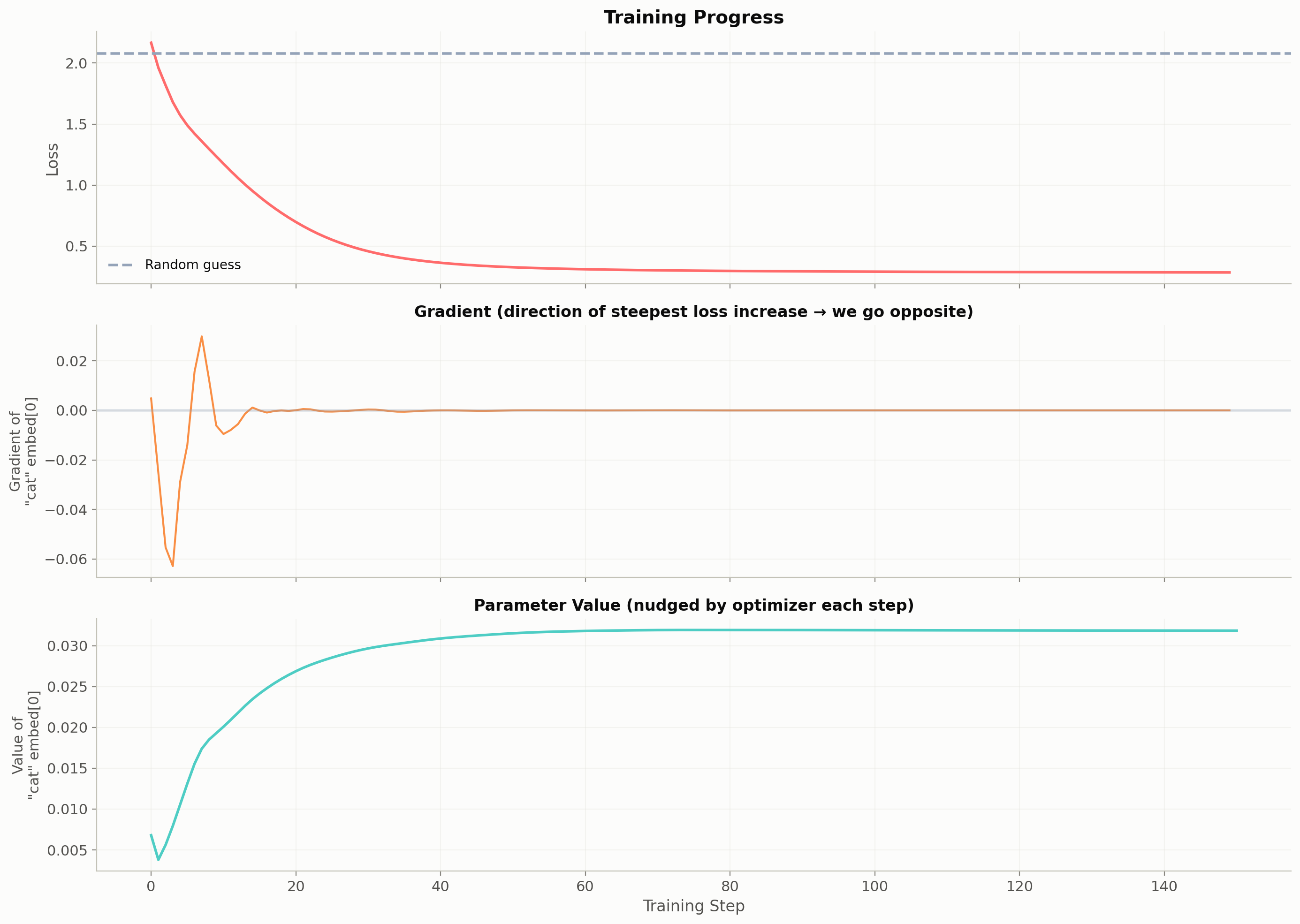
Gradients tell us the slope of the loss landscape — which direction to move each parameter to reduce the loss. The optimizer takes a step in that direction.
Let’s watch a single parameter (one value in the embedding of “cat”) as we train.
Show plotting code
# Reset model for clean trackingtorch.manual_seed(42)model = Transformer(config).to(device)optimizer = torch.optim.AdamW(model.parameters(), lr=3e-3)# Track one specific parameter over trainingparam_idx = (tok2id['cat'], 0) # first dimension of "cat" embeddingparam_history = []loss_history = []grad_history = []n_steps =150model.train()for step inrange(n_steps): logits = model(train_x) loss = F.cross_entropy(logits.view(-1, vocab_size), train_y.view(-1)) optimizer.zero_grad() loss.backward()# Record before optimizer step param_val = model.tok_embeddings.weight[param_idx[0], param_idx[1]].item() grad_val = model.tok_embeddings.weight.grad[param_idx[0], param_idx[1]].item() param_history.append(param_val) loss_history.append(loss.item()) grad_history.append(grad_val) optimizer.step()# Final valueparam_history.append(model.tok_embeddings.weight[param_idx[0], param_idx[1]].item())fig, axes = plt.subplots(3, 1, figsize=(14, 10), sharex=True)# Loss over timeaxes[0].plot(loss_history, color='#FF6B6B', linewidth=2)axes[0].axhline(y=np.log(vocab_size), color='#94A3B8', linestyle='--', label='Random guess')axes[0].set_ylabel('Loss', fontsize=12)axes[0].set_title('Training Progress', fontsize=14, fontweight='bold')axes[0].legend(fontsize=10)axes[0].grid(True, alpha=0.3)# Gradient over timeaxes[1].plot(grad_history, color='#F97316', linewidth=1.5, alpha=0.8)axes[1].axhline(y=0, color='#94A3B8', linestyle='-', alpha=0.3)axes[1].set_ylabel(f'Gradient of\n"cat" embed[0]', fontsize=11)axes[1].set_title('Gradient (direction of steepest loss increase → we go opposite)', fontsize=12)axes[1].grid(True, alpha=0.3)# Parameter value over timeaxes[2].plot(param_history, color='#4ECDC4', linewidth=2)axes[2].set_ylabel(f'Value of\n"cat" embed[0]', fontsize=11)axes[2].set_xlabel('Training Step', fontsize=12)axes[2].set_title('Parameter Value (nudged by optimizer each step)', fontsize=12)axes[2].grid(True, alpha=0.3)plt.tight_layout()plt.show()print(f'"cat" embedding[0] moved from {param_history[0]:.4f} to {param_history[-1]:.4f}')print(f'That\'s a total shift of {abs(param_history[-1] - param_history[0]):.4f}')
"cat" embedding[0] moved from 0.0068 to 0.0318
That's a total shift of 0.0250
🏗️ Project milestone M4 — first training run
Point this chapter’s training loop at your model: load checkpoints/myllm/config.json, build the Transformer, and train 300 steps on this chapter’s dataset. Save the loss curve and the checkpoint:
Accept when: loss is clearly decreasing (final < 60% of initial) and step300.pt reloads into a fresh model without key errors. Part of The Project: Serve Your Own LLM.
Sessions S2.2–S2.3 split this milestone: M4a (S2.2) is a 20-step smoke run saved to loss_smoke.json (a JSON list of losses), with the 300-step run launched at session’s end; M4b (S2.3) verifies step300.pt + loss_step300.json. Verify: uv run pytest tests/milestones/.
Key Takeaways
Training = forward → loss → backward → update, repeated. That’s the entire algorithm.
Cross-entropy loss = -log(probability of correct token). Lower = model is less surprised.
Gradients point toward steeper loss — the optimizer steps in the opposite direction.
Each parameter gets its own gradient — the model has thousands of knobs being tuned simultaneously.
Next notebooks
01_learning_rate_schedules.ipynb — why LR matters and how cosine annealing works
02_mixed_precision.ipynb — train 2x faster with half-precision floats
03_gradient_accumulation.ipynb — simulate large batches on small hardware
04_adamw_from_scratch.ipynb — build the optimizer step by step